1-2. Oceanic cycle model

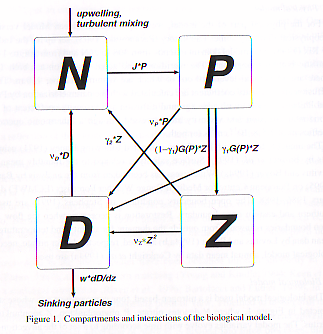
a. Summary

The simple marine ecosystem model with four ingredients was included in the oceanic circulation model COCO which the University of Tokyo climate center and an earth frontier develop jointly, and the result of having performed integration for seven years was compared with observational data. The mixolimnion depth which is physical environment important for a marine ecosystem is comparatively often reproduced by the general circulation model, and the mixolimnion depth seasonal variation with the big amplitude in northern North Atlantic Ocean and the Antarctic Ocean is also expressed by the model. Moreover, the phenomenon in which the bloom of phytoplankton happened for the rapid change of the mixolimnion depth in signs that concentration becomes high also about the chlorophyll concentration distribution used as the index of a phytoplankton standing crop by northern North Atlantic Ocean and North Pacific, an equatorial region, and Ekman upwelling called the Antarctic Ocean, northern North Atlantic Ocean, and the Antarctic Ocean etc. was reproduced by the model. It has already completed and inclusion to the model of a carbonic-acid system is also due to perform integration for thousands of years required to reach regularly after this. In order to perform such long-term integration under a setup by this research which can be called high resolution as a marine ecosystem model of all balls, even if it uses an Earth Simulator, the real time for about three months is required, and in the conventional supercomputer, it can be said that it is impossible as a matter of fact.

b. Research purpose

The total carbonic acid vertical distribution in the ocean is carrying out characteristic distribution to which concentration becomes low near a surface. Such distribution with the big meaning for air sea exchange of carbon dioxide is determined by process, such as a living thing pump alkali pump and a physical pump, and is making contribution with the most important living thing pump resulting from sedimentation which follows the formation and it of an organic matter in a surface ecosystem especially. The efficiency of the living thing pump is influenced by various physical process, such as the depth of a sea mixolimnion, and transportation of the iron by Ekman upwelling and the atmosphere. Therefore, the climate change resulting from artificial origin carbon dioxide changes a living thing pump, and there is a possibility of enough of bringing positive or negative feed back further to carbon-dioxide absorption of the ocean.

According to the result of the terrestrial-air-sea combined carbon circulation model which a Hadley-center (English) and IPSL (France) performed, influence which a climate change has on carbon-dioxide absorption of the ocean is made small (Cox et al., 2000; Friedlingstein et al.2001). However, according to change of the sea carbon-dioxide absorption computed from the inversion calculation based on the carbon-dioxide-levels distribution in the atmosphere, or observation of the nitrogen / oxygen ratio in the atmosphere, it is suggested that the present sea carbon cycle model has the blunt sensitivity to a climate change. For prediction of the carbon dioxide levels in the atmosphere, it is required to improve a sea carbon cycle model succeedingly. In this subject of research, the simple marine ecosystem model of four variables is included in an oceanic circulation model with a carbon cycle model, the interaction of a sea carbon cycle and a climatic change is investigated, and it aims at developing further and studying construction of a terrestrial-air-sea combined carbon circulation model, and all the ball scale carbon cycles by it.

c. A research program, a method, a schedule

the phytoplankton according to Oschlies and Garcon (1999) as an ecosystem model included in an integrated model sea carbon cycle component, nitric acid, a zooplankton, and Deet Wrye -- 4 compartment surface ecosystem model which makes TASS a variable is considered (Fig. 1).

Fig. 1: Key map of marine ecosystem model to adopt. As for N, nitric acid and P express phytoplankton, Z expresses animal plankton, and D expresses detritus, respectively.

The model with the complicated structure where the structure of an actual ecosystem is more faithfully reproduced by many researchers other than such a model is developed, and the uncertainty of a parameter [ in / moreover / including many constituent factors / besides a marine ecosystem model / each ] of the integrated model which should finally be developed is also large. In such a situation, it judged that it was not a best policy to introduce the marine ecosystem model which has not much complicated structure in the present stage, and decided to adopt the four above-mentioned compartment models. A carbon-dioxide gradual increase experiment is due to perform immediately inclusion to the general circulation model of this model, and to be conducted by 3rd using the joint model which incorporated the terrestrial carbon cycle model further.

In the 3rd and afterwards, while performing experiment which used this joint model, and analysis of a result, it considers building the latest model also in consideration of the effect of air transportation of iron. The marine ecosystem model which adopted the iron effect is already developed partly (e. g., Leonard et al., 1999; Archer and Johnson 2000; Moore et al, 2002), and it is thought that it is possible enough to make our model to reference and to change them into it. Moreover, about air transportation of iron, it already exists in the form where the dust transportation model which one of research implementation persons developed is immediately included in a general circulation model. The influence which the iron transportation by the atmosphere has on a living thing pump can be explicitly dealt with now by combining these, and coming that it can perform a more concrete argument about the feedback mechanism (Kumar et al.1995) through the iron proposed about a glacial-interglacial cycle or global warming is expected.

d. The research program in FY 2002

The suitable model including a simpler process (about four ingredients) for the side and the integrated model which further development of a model including detailed living thing and geochemistry process (ten or more ingredients) advanced in the global warming region of prediction is built about a sea carbon cycle, and the work introduced into the inside resolution version of oceanographic model COCO developed in the University of Tokyo climate center is started.

e. Reports in FY 2002

Inclusion of the marine ecosystem model to COCO was finished, and comparison with the preliminary result and the observation which are depended on a model was performed (Fig. 2 - figure 4). It supposes that a comparison result is stated by "f. consideration", and, below, it describes the outline of a model.

As mentioned above, it is as an ecosystem model. The thing of Oschlies and Garcon (1999) is used. This model has four, nitric acid (N), phytoplankton (P), animal plankton (Z), and detritus (D), as a forecast variable, and each amount of existing is expressed with a nitrogen base. Time development of a variable is what added the sauce sink clause which expresses the interaction between variables with an advective diffusion equation, and is described. In the parameter values of a model, it is fundamentally. The same thing as Oschlies and Garcon (1999) is given. However, correction was added to sedimentation of detritus, and the handling of a photosynthetic rate. Oschlies and Garcon (1999) is sedimentation velocity fixed in all layers. Although 5 m/d was given, it is a surface here. It is sedimentation velocity to 150m. It sediments by 5 m/d and is in a place deeper than it. It was presupposed that it is distributed in the perpendicular direction of detritus sedimentation flux according to the curve which Martin (1987) advocated. Again Oschlies and Garcon (1999) had adopted. About the temperature dependency of the photosynthetic rate by Eppley (1972), there shall be no 20-degree C temperature dependency in the above domain. What Wanninkhof (1992) formulized was used about the piston speed in the case of the carbon dioxide exchange between the air-oceans. About the sedimentation process of calcium carbonate husks, it was dealt with like the thing about detritus.

Horizontal resolution of the oceanic circulation model COCO was set into 1 degree, and the perpendicular number of layers set east and west to 54. It was made what ten layers are set for from 20 layers and 100m by 200m on 100m of surfaces among them. As a mixolimnion model Mellor and Yamada (1974) The closure scheme of level 2 is used. Wind stress, sea surface heat and freshwater flux, and surface boundary condition of insolation What is distributed by OMIP (Ocean Model Intercomparison Project, http://www.clivar.org/organization/wgomd/pomip-e.htm) was adopted.

In the initial value at the time of integrating with a model, it is about nitric acid. The climate value data based on Conkright (1998) was used. phytoplankton, a zooplankton, and Deet Wrye -- TASS -- all layers It was considered as 0.1 mmol/m³. Since a climate value data set like [ alkalinity / a total carbonic acid and ] nutrient salt did not exist for the moment, steady value 2000 mol/m³ was given to all layer 1 [ Mr. ]. Probably these variables have distribution with perpendicular and a horizontal direction significant in a nature, and like an experiment here, as a preliminary experiment, it will be enough [ giving a steady value to all layers ], although it is a setup which is originally hard to accept, when an integration period is short. The place which found the integral to the general circulation model for 10,000 years, without combining with an ecosystem model, and reached the steady state was given, and it was considered as the initial value. Seven-year part integration is performed from the above initial value, and the obtained analysis result about the 7th year is shown in the following paragraph.

f. Consideration

February to April (FMA)	May to July (MJJ)
August to October (ASO)	November to January (NDJ)

February to April (FMA)	May to July (MJJ)
August to October (ASO)	November to January (NDJ)

Fig. 2: Seasonal variation of mixolimnion depth. Model result (a) Climate value data (b) . Unit m.

The depth of the mixolimnion which a general circulation model reproduces is a factor important for an ecosystem model in order to specify the light environment and nutrient salt environment of phytoplankton. In Fig. 2, comparison with a model and observation is performed about the seasonal variation of a mixolimnion. The density variations over a sea surface make the definition of a mixolimnion water temperature here. 0.5 It was considered as the depth which reaches the value corresponding to a degree. The mixolimnion of observation was calculated based on the data of the water temperature and salt of Conkright et al. (1998). Moreover, since the seasonal variation of sea water temperature was in a phase about two months compared with atmospheric it, seasonal paragraph classification defined February to April as winter (referred to as FMA in the summer of the Southern Hemisphere) of the Northern Hemisphere, and defined it as - autumn (autumn of the Southern Hemisphere - winter - spring respectively MJJ-ASO-NDJ) below in the summer of - in the spring of the Northern Hemisphere every three months. It turns out that the model is often reproducing signs that a mixolimnion becomes northern North Atlantic Ocean by FMA, and becomes deep to about 500m by ASO in the Antarctic Ocean. However, in the model result, the mixolimnion is deeper, and the area of the domain where a mixolimnion is deep is also large. It is because this compensates and has the vertical distribution of water temperature and salt in a part in a model and perpendicular uniform density distribution is formed, and it is not necessarily shown that the range where mixture reaches in a model is too deep. In order to express faithfully the range where mixture reaches in a model, it was desirable to define the depth of a mixolimnion on the basis of a perpendicular diffusion coefficient, but correspondence with the mixolimnion depth calculated from observational data was considered, and the above-mentioned definition was adopted here.

The seasonal variation of the sea surface chlorophyll concentration used as the index of a phytoplankton standing crop is shown in Fig. 3 about a model result and satellite observation (CZCS). In addition, scaling ratio fixed for obtaining chlorophyll concentration from a model result 1.59/(mg/m³) (mmol/m³) was used. Through every year, a model is sufficient as the situation that concentration is high, and it is reproduced in northern North Atlantic Ocean and North Pacific, an equatorial region, and the Antarctic Ocean. This is because the nutrient salt supply from a lower layer is prosperous in these ocean space because of Ekman upwelling. Moreover, it turns out that the bloom phenomenon in which light environment is improved in MJJ to which a mixolimnion becomes shallow rapidly in northern North Atlantic Ocean, and chlorophyll concentration becomes high rapidly is caught also for the model. Although overestimation in an equatorial region is most conspicuous by the difference between a model and observation, this is bias seen in common with other large-scale scale marine ecosystem models (Fasham et al., 2001), and needs to tackle the removal over many hours after this.

The amount of air-sea carbon dioxide exchange which carried out year-round integration was shown in Fig. 4. Since the integration period is as short as seven years, it depends for a model result to an initial value strongly. Although the result of this experiment which gave a total carbonic acid and alkalinity uniformly with all balls is seen scientifically and is not so much meaningful, it will be meaningful as what shows the development phase of a model. Henceforth, integration for thousands of years required to reach regularly is due to be performed. When integrating with a general circulation model after combining a marine ecosystem model The accelerated method of Bryan (1969) cannot be used but a great quantity of calculation resources are needed for long-term integration. It is impossible it to be expected for that it takes the real time for three months or more even if it uses an Earth Simulator for performing thousands of years of integration by setup in this experiment, and to carry out with the conventional supercomputer as a matter of fact. A great contribution is expectable to an understanding of a sea carbon cycle by using an Earth Simulator.

February to April (FMA)	May to July (MJJ)
August to October (ASO)	November to January (NDJ)

February to April (FMA)	May to July (MJJ)
August to October (ASO)	November to January (NDJ)

Fig. 3: Seasonal variation of sea surface chlorophyll concentration.
Model result (a) Satellite observation by CZCS (b). Unit mg/m³.

g. Bibliography

h. The announcement of a result