1-2. Oceanic carbon cycle model

a. Summary

As a preceding paragraph story of carbon cycle process inclusion to an air sea joint model, the preliminary warming experiment was conducted using the carbon cycle model included in the sea simple substance model. That is, it was investigated how the amounts of sea carbon dioxide absorption when the carbon dioxide levels in the atmosphere increase gradually about the case where marine environment changes with warming, and the case where that is not right, using the wind stress and sea skin temperature which were obtained as a result of the carbon dioxide gradual increase experiment conducted in the past using the air sea joint model as driving force of a sea model would differ among both cases. Consequently, the result that the influence which the sea circulation change by warming has on the amount of carbon dioxide absorption was small was obtained. The model adopted in this project finished with the warming experiment here confirming the past experimental result, although description of a sea surface ecosystem was detailed rather than what is adopted by the IPCC Third Assessment Report. Although this very thing is not a gay result, it can be said that it has checked that our model showed the behavior which will seemingly be reasonable as a preceding paragraph story combined with terrestrial carbon cycle. This is received, a carbon cycle model transplant to an air sea joint model is also started, and it is in the stage which the prototype completed now. From now on, tuning of a model parameter, maintenance of a code, and sufficient spin rise are performed, and it will prepare for the participation to both the carbon cycle-climate joint model comparison project (C4MIP), as a result the contribution to the 4th IPCC report. Furthermore, the experiment using the model which expressed the seed composition of a plant and animal plankton explicitly was also conducted, and it investigated about the influence which seasonal perpendicular movement of copepod and the climate change of a ten-year scale have on a sea surface ecosystem.

b. Research purpose

All lead carbonate direct distribution in the ocean is carrying out characteristic distribution to which concentration becomes low near a surface. Such distribution with the big meaning for air sea exchange of carbon dioxide is determined by process, such as a living thing pump alkali pump and a physical pump, and is making contribution with the most important living thing pump resulting from sedimentation which follows the formation and it of an organic matter in a surface ecosystem especially. The efficiency of the living thing pump is influenced by various physical process, such as the depth of a sea mixed layer, and transportation of the iron by Ekman upwelling and the atmosphere. In order to grasp how much the carbon dioxide discharged by human activities remains in the atmosphere and to make probable prediction of the future carbon dioxide levels in the atmosphere, it is indispensable to model the carbon cycle process in the ocean exactly.

According to the result of the terrestrial-air-sea combined carbon circulation model which a Hadley center (English) and IPSL (France) performed, influence which a climate change has on carbon dioxide absorption of the ocean is made small (Cox et al., 2000; Friedlingstein et al.2001). However, when the result submitted to both the sea carbon cycle model comparison project (Ocean Carbon-Cycle Model Intercomparison Project, OCMIP) is seen, in the amount future prediction of sea carbon dioxide absorption of a baseline performed without taking a climate change into consideration, the variation between models is large and the predicted value in the 2100 time has a twice as many difference as this between the minimum value and maximum (Fasham, 2003). For prediction of the carbon dioxide levels in the atmosphere, it is required to improve a sea carbon cycle model succeedingly and to reduce such uncertainty. In this subject of research, the simple sea ecosystem model of four variables is included in an oceanic circulation model with a carbon cycle model, the interaction of sea carbon cycle and a climatic change is investigated, and it aims at developing further and studying all ball scale carbon cycle by construction and it of a terrestrial-air-sea combined carbon circulation model.

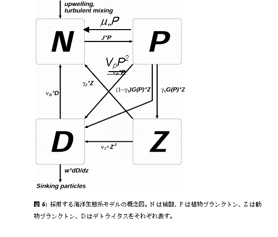
c. A research program, a method, a schedule

As an ecosystem model included in an integrated model sea carbon cycle component, it is Oschlie to the phytoplankton by Oschlies and Garcon (1999), nitric acid, animal plankton, and 4 compartment surface ecosystem model of detritus. It carries out (Fig. 6).

d. The research program in FY 2003

The work which combines a sea carbon cycle model and a terrestrial carbon cycle model with the air sea joint climate model MIROC is started during the current fiscal year. About the sea component, combination with an ecosystem model with four simple ingredients and an oceanic circulation model is completed mostly. About a terrestrial component, inclusion to the climate model of Sim-CYCLE under development is started by an earth frontier research system at the beginning of FY 2003. Integration of the land process model MATSIRO and Sim-CYCLE is also performed. Moreover, in order to be anxious about vegetation distribution changing with warming sharply about a subarctic zone wood, development of the vegetation dynamic model which specialized in the subarctic zone wood towards Sim-CYCLE extension is begun. Before including in MIROC, it is necessary to fully perform examination of the performance in each component model simple substance.

e. Reports in FY 2003

Inclusion of the sea ecosystem and carbon cycle model to the oceanic circulation model COCO was finished in FY 2002, in the current fiscal year, the model was run also as that of some different forcing, and the performance check was performed. After the model checked showing the behavior which will seemingly be reasonable, carbon cycle model inclusion was tackled at the air sea joint model MIROC. It is in the state where the prototype of the carbon cycle-climatic change joint model containing the carbon cycle of terrestrial and the ocean was completed at present. This section describes the result of the comparison with the time of using the time of using the thing based on observation for sea surface model driving force called a sea surface water temperature and salt, and wind stress which performed the model performance check as a main purpose, and a joint model output, and a future prediction experiment of the amount of b human work origin carbon dioxide sea absorption below. Comparison like a is performed in order to verify the validity of driving a sea model with the output of an air sea joint model by b.

An ecosystem model is as above-mentioned. Oschlies (2001) uses for the model of Oschlies and Garçon (1999) what added improvement. A thing is used. A carbonic acid system chemical process is introduced according to the protocol which both the sea carbon cycle model comparison project (Ocean Carbon Cycle Model Intercomparison Project, OCMIP) recommends to this ecosystem model, and the carbon cycle in the ocean is described. The horizontal resolution of the oceanic circulation model COCO (Hasumi, 2000) which carries this carbon cycle model is 1 time, and east and west and the north and south of the perpendicular number of layers are 54. About the details of a model, especially an ecosystem model should refer to description by Oschlies and Garçon (1999) with the result report in FY 2002.

The monthly average data distributed as drive data based on observation about the comparative experiments of a. corresponding to both the sea model comparison project (Ocean Model Intercomparison Project, OMIP) is used. The drive data based on a model output is created based on the result submitted to the IPCC Third Assessment Report (IPCC, 2001) using the air sea joint model (horizontal resolution is the atmosphere T21 and about 2.8 oceans) of CCSR/NIES. That is, the output data which took the average about 60 years from 1851 of an experiment start to 1910 the signs of warming will begin to be in sight is used as driving force for sea models. As carbon dioxide levels in the atmosphere, the value of 280 ppm before the Industrial Revolution is given. Hereafter, the thing based on experiment A1 and a model output for the experiment based on observation will be called experiment A2.

the thing (experiment B1) using the time series of the warming prediction experimental result according to a joint model to driving force as a future prediction experiment of the amount of carbon dioxide sea absorption of b., and the thing (experiment B-2) using a seasonal variation fixed every year -- two kinds are performed. By comparing the result of B1 and B-2, the knowledge about influence which change of the marine environment by warming brings to the carbon cycle in the ocean can be acquired. The same thing as A2 is used for the driving force of B-2. The result of the warming experiment by the CCSR/NIES model described in the top is directly used for the driving force of B1. About the carbon-dioxide-levels scenario in the atmosphere, till 1990, B1 and B-2 gave the time series based on an observed value, and assumed that it increased gradually henceforth by a unit of 1% every year. As mentioned above, the conclusion of the conducted experiment is hung up over Table 1.

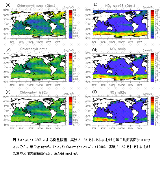
The integration procedure of experiments A1 and A2 is described below. As an initial value of water temperature and salt, the annual average climate value according the integration result for 10,000 years which Nakano (2000) performed to Conkright et al. (1994) about nitric acid is given, respectively. Moreover, about all carbonic acids and alkalinity, the regular value acquired by the model of Yamanaka and others (Orr, 2002 references) corresponding to both the sea carbon cycle model comparison project (Ocean Carbon-Cycle Model Intercomparison Project, OCMIP) is used as an initial value. About variables other than the nitric acid of an ecosystem model, steady value 0.1 mmol/m³ was given as an initial value. A1 and A2 from this state -- integration is performed for 19 years using each driving force, and it analyzes about the result for [ of the last ] one year. In addition, although the integration period of 19 years is too short for attaining a perfect stationary state, in order to remove the shock immediately after an integration start, it is sufficient period, and the result obtained deserves the analysis for a performance check enough.

About B1 and B-2, the integration result of A2 is made into an initial value, the surface driving force corresponding to each and the carbon dioxide levels in the atmosphere are given, and it finds the integral from 1851 to 2100. Below, first, A1 and A2 are compared and it is examined how appropriate it is to use the result of a joint model as driving force of a sea simple substance model. The result of B1 and B-2 is described after that, and future prediction of the amount of artificial origin carbon dioxide sea absorption and change of the marine environment by warming argue about the influence which it has on carbon cycle.

Fig. 7 shows the result of experiments A1 and A2, and an observed value about the sea surface chlorophyll and nitric acid concentration of an annual average. In addition, for obtaining chlorophyll concentration from a model result, fixed conversion ratio 1.59(mg/m³)/(mmol/m³) was used.

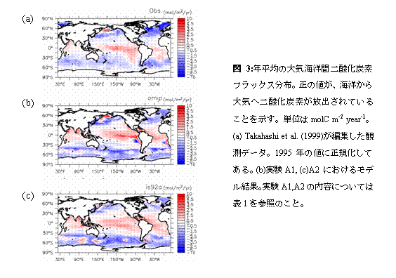
It will see about chlorophyll concentration first. Experiments A1 and A2 show a high value in subarctic zone JAIA of northern North Pacific and North Atlantic Ocean, the Antarctic Ocean, and an equatorial region, and this is in agreement with the feature looked at by satellite observation. However, especially about the maximum of an equatorial region, both experiments show the high value compared with satellite observation in the Pacific Ocean. This is bias looked at by all other ball scale scale sea ecosystem models (Fasham et al.2001), and needs to tackle the removal over many hours after this.

When A1 and A two-car experiment are compared, it turns out that chlorophyll concentration shows the result of having also born a strong resemblance to a value and distribution. The point which the maximum of the Pacific Ocean equatorial region in A1 says that north-south width is larger than the thing of A2 as a conspicuous difference is mentioned. Especially this tendency is remarkable in an eastern equatorial region. This originates in a more strong thing in the wind stress which the trade winds which bring about equatorial upwelling in this ocean space gave to the experiment A1. Moreover, in the experiment A1, coast upwelling strong off Peru is excited so that it may state later, and this has also become the cause that such a difference is seen in an eastern equatorial region.

Next, it sees about distribution of nitric acid concentration. In the climate value by Conkright et al. (1998), a high value is seen in subarctic zone JAIA of northern North Pacific and North Atlantic Ocean, the Antarctic Ocean, and an equatorial region, and such a feature is roughly reproduced also in A1 and A two-car experiment. However, in the experiment A2, the concentration of the nitric acid maximum in a Pacific Ocean equatorial region is underestimated. In addition, on a setup of a color scale, although the nitric acid maximum of a Pacific Ocean equatorial region has disappeared in A2, the weak maximum exists in fact as reflected in chlorophyll concentration distribution (figure 2e). Moreover, in the experiment A1, nitric acid concentration is high notably on the Peru coast. Since the ingredient along the shore of the wind stress in this ocean space is larger in what was given to the experiment A1, this originates in strong coast upwelling being excited. The typical value of the coast upwelling speed in this ocean space actually reaches 1 m/day. In the model of coarse lattice size which has been adopted here, the maximum of coast upwelling speed tends to be underestimated and a upwelling speed called 1 m/day which is equal also to equatorial upwelling can be said to be a very large thing. It is the unreal formation factor here of the nitric acid maximum which "the nutrition salt capture (nutrient trapping)" which Maier-Reimer (1993) pointed out as an unreal formation factor of the sub surface Lynn acid maximum in an eastern Pacific Ocean equatorial region generated also in coast upwelling tact. The direction of the driving force of A1 based on an observed value has brought about the unreal calculation result about the point described here.

It is the nitric acid concentration in the Pacific Ocean sector of the Antarctic Ocean which should be pointed out to others among the differences between both experimental results. Also in A2, the direction is small notably. This is because the winter mixed layer of the Antarctic Ocean is shallow by A2. The rain of a model has increased in this ocean space compared with objective-analysis data, sea surface salt is stopped low, and it is because the convection has stopped being able to happen easily that a winter mixed layer becomes shallow by the driving force of A2 based on a joint model output. In addition, it is thought that a Ekman upwelling style also has big influence on the sea surface nitric acid concentration in this ocean space. However, in this case, the Ekman upwelling style calculated from wind stress is strong rather in the experiment A2, and this is contradictory to the sea surface nitric acid concentration of A2 being low. It turns out that the difference in a Ekman upwelling style did not bring about the difference between 2d of figures, and the Antarctic Ocean surface nitric acid concentration of f.

Each result of the observation data gathered by Takahashi et al. (1999) and experiments A1 and A2 was shown in Fig. 8 about the amount of carbon dioxide exchange between the air oceans. However, it will be normalized as of 1995 and the distribution by Takahashi et al. (1999) cannot compare the value of 280 ppm before the Industrial Revolution as carbon dioxide levels in the atmosphere the result of A1 and A2 which were given and obtained, and directly. Having hung up figure 8a should catch to the last for reference of a near distribution and value.

Fig. 8 Comparison of b and c looks at the difference in the carbon dioxide discharge to which the direction of A1 met the equator in figure 8b in the Pacific Ocean equatorial region corresponding to upwelling being strong being strong from the thing in figure 8c etc. However, rather than the impression acquired from comparison of the experiments A1 and A2 in Fig. 7, it could be said that the result of figure 8b and c resembles each other. There is total carbonic acid concentration as one of important elements which determines the amount of carbon dioxide exchange between the air oceans. Although the total carbonic acid concentration and nitric acid concentration have the dynamic state which could lead the Redfield ratio and was alike, such a difference arises, in order that the feedback which led may commit the air sea carbon dioxide exchange itself. It explains taking the case of the Antarctic Ocean. As shown in 7f of figures, when a winter mixed layer is shallow and nitric acid is not carried to a surface, all carbonic acid transportation from the depths also becomes less than a mixed layer. Consequently, although carbon dioxide partial pressure on the surface of the sea also becomes low then, carbon dioxide partial pressure differential with the atmosphere becomes large, and the carbon dioxide flux which goes to the ocean from the atmosphere increases. In this way, the total carbonic acid concentration, as a result carbon dioxide partial pressure near a surface will increase, and the amount of carbon dioxide exchange of the Antarctic Ocean will not change so much between figure 8b and c as a result. Since such a feed back mechanism exists, even if the carbon dioxide exchange between the air oceans shows the distribution which was alike between figure 8b and c, the income and outgo of all the carbonic acids near a mixed layer may be greatly different.

e.1. The time series of the amount of sea carbon dioxide absorption which carried out all ball integration is shown in Fig. 9 about the experiment B1 conducted according to the procedure stated in the paragraph, and B-2. In the experiment B1, everything but the thing of the climate made within a joint model seen for change by the amount of carbon dioxide absorption every year corresponding to change of both of experimental results is very well alike. B1 and B-2 of the flux in the 2100 time are 5 PgC/year remainders, and the difference during both experiments is about 0.5 PgC/year.

The influence which the sea circulation change by warming has on the amount of carbon dioxide absorption in the experiment using this model is small so that it may understand from here. The result of having conducted the experiment even with the IPCC Third Assessment Report same at two or more models is reported, and according to it, a difference has the influence of warming by a model. However, compared with the result of having conducted the experiment which corresponds by a terrestrial carbon cycle model, the influence of the sea carbon cycle on warming is small intentionally, and every sea model can be said that our result is not contradictory to the past thing at this point. The model adopted in this project finished with the warming experiment here confirming the past experimental result, although description of a sea surface ecosystem was detailed rather than what is adopted by the IPCC Third Assessment Report. Although this very thing is not the result of attracting attention, it can be said that it has checked that our model showed the behavior which will seemingly be reasonable as a preceding paragraph story combined with terrestrial carbon cycle.

However, as compared with the model result published by the IPCC Third Assessment Report, the result in this model belongs to a category with the small influence of warming. That is, intuitively, in order that the ocean may get warm at experiment B1, carbon dioxide partial pressure in the ocean becomes high, and is considered that the amount of carbon dioxide absorption becomes less rather than B-2 as a result. Although the direction of B1 is actually small even in Fig. 9 in the amount of absorption, the following points can be considered as a reason in the tendency for the difference to be smaller than the model of other IPCC Third Assessment Reports. :

Fig. 12: Difference of living thing primary manufacturing which carried out annual average when not considering it as case where copepod carry out seasonal perpendicular movement (mgC/m²/d). When the value of plus carries out perpendicular migration, it is shown that a living thing primary manufacturing becomes high.

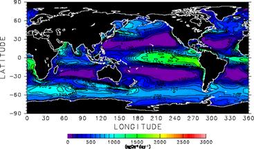
This fiscal year also conducted the secular change reappearance experiments from 1948 to 2002. marine [ where this is offered as a NCEP re-analysis data set ] -- it is the calculation which drives Global COCONUTS by making Japanese average value, such as temperature, wind stress, Amount of insolation, precipitation, and the amount of evaporation, into external force. The living thing primary manufacturing which averaged full time integration period 54 years is reproducing the distribution which says roughly and is obtained by observation of taking a high value, a value low in a subtropical region, etc. on the North Pacific subarctic zone region, a south ocean, the equator, etc. (Fig. 13). However, since iron restrictions etc. are not taken into consideration in the present version, it is overestimation in a south ocean or the equatorial Pacific Ocean. This is the point which should be improved promptly.

f. Consideration

(a) PDO(s) (Pacific Decadal Oscillation) from figure 14:1950 to 2002 Deviation from the average value of the living thing primary manufacturing in Index and (b) North Pacific Midwest (%)

Fig. 15: Difference of living thing primary manufacturing for ten years each (1977 - 1985 [ 1964 - 1975, ]) before and behind climate jump (mgC/m²/d). It is shown that the quantity of production after a climate jump increased the value of plus.

g. Bibliography

h. The announcement of a result