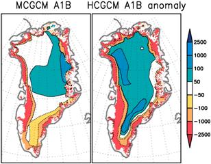
a. Summary

In order to investigate the influence of the response characteristic and sea level on the ice sheet to warming, inclusion of the ice sheet model to presumption by a high resolution air sea joint model, presumption which inputted the air oceanographic model result into the ice sheet model, and an earth system model including a carbon cycle, and the uncertainty factor of the model about ice sheet change were examined. MIROC3.2 In the SRES scenario (A1B and B1) warming experiment using the high resolution version and the inside resolution version, the contribution to the sea level of Greenland and the South Pole ice sheet became 15cm rise in the sea level and 5cm sea surface fall by the high resolution model respectively, and it turned out that being smaller than sea thermal expansion and an advanced change tendency can obtain the result which does not have the latest observation fact and inconsistency. Furthermore, it is CO2 in order to investigate long-term influence. The air sea joint model experimental findings which continued giving the concentration of an increase experiment or a SRES scenario 4 times were inputted into the ice sheet model (Saito and Abe-Ouchi, 2004, 2006) developed so that reality might often be expressed. In 4 redoubling experiments of CO2, the Greenland ice sheet will disappear mostly about in 2000, and sea levels are a 6m upsurge and SRES. When the result which the end or subsequent ones of the 21st century continued giving the concentration of a scenario in 200 was used, it turned out that long-term reaction continues compared with the case where temperature is fixed at the end of the 21st century, and an ice sheet finally disappears. In order to clarify uncertainty of an ice sheet model, no less than two points, the numerical technique and a mass income-and-outgo model, were examined, and the grade of the uncertainty on the conditions which result in ice sheet disappearance was also clarified. It ends mostly and the program alteration for enabling calculation of air-ice sheet combination (partial integrated model) which synchronized is continuing the present adjustment.

b. Research purpose

An ice sheet is ashore, there is sea ice in earth top north-south two poles at sea, and those generation change is directly linked with the climate change of an earth scale. For this reason, in connection with warming, an ice sheet and sea ice react sensitively, and we dissolve, or are anxious about affecting still wide range climate and sea surface change. So, into this group, the atmosphere / ocean / sea ice / ice sheet joint model which finally works on an Earth Simulator are built, and the prediction experiment of global warming or sea surface change is conducted. First, it strives for grasp of an indefinite element through various sensitivity experiments, improving a partial model. Furthermore, it aims at raising the accuracy of a prediction experiment, conducting the reappearance experiment of the present or the past using the combined model. Moreover, since the past climate and the restoration of ice sheet change / sea level by the data of a seabed sediment or geographical feature have come to be considerably performed with high precision about the last glacial epoch or subsequent ones 20,000 years ago, the model is verified through trying the numerical simulation reproducing this.

c. A research program, a method, a schedule

About the ice sheet, manufacture of a partial model was briefly performed by the 14 fiscal year, and the response characteristic has been investigated. In the 15 fiscal year, improved each portion or the parallelization optimization of the ice sheet model program was carried out for Earth Simulators, and the coupling agent was developed and the characteristic of combination of a climate model and an ice sheet dynamics model was investigated. The warming experiment was conducted using the air sea joint model of the resolution of a degree in the middle, and the influence on sea ice or an ice sheet was considered in the 16 fiscal year and the 17 fiscal year. From now on, combination of an ice sheet model and an air model is completed, and warming influence is discussed quantitatively.

d. The research program in the Heisei 17 fiscal year

Verification through observational data or a paleoclimate reappearance experiment was performed in the last fiscal year, and highly precise-ization of the ice sheet model developed in the University of Tokyo climate center and the sea ice model introduced into MIROC has been performed. It is doing a numerical simulation which combined these air sea sea ice joint general circulation models and ice sheet models, and examination will be begun for what kind of influence the chill areas, such as an ice sheet of the South Pole or Greenland and sea ice, receive in global warming in the 17 fiscal year. CO2 When a greenhouse gas level is stable even by about 4 times, it is due to integrate with how climate and an ice sheet answer over a long period of time for hundreds years, and to experiment in it.

e. Fruits of work in the Heisei 17 fiscal year

It considered further how the uncertainty of the warming experiment by a climate model would influence ice sheet change with various time factors as the input of an ice sheet model using the result of a warming experiment of a symbiosis first division title, and the warming response of the Greenland ice sheet was investigated.

MIROC3.2 Place which carried out interpolation of the result of the SRES scenario (A1B and B1) warming experiment using the high resolution version and the inside resolution version to the ice sheet form of observation, and analyzed it in detail (it is Compensation Wild et al about the ice sheet form of GCM being too coarse) (2000), Respectively, by the high resolution model, the contribution to the sea level of Greenland and the South Pole ice sheet became 15cm rise in the sea level and 5cm sea surface fall, respectively, and brought a result smaller than sea thermal expansion (Fig. 36, Suzuki et al, 2005). The Greenland ice sheet is because the volume increase by the increase in precipitation is effective in the South Pole for the time being, although dissolution stands high by warming. The thing with small diversification is for the reaction of an ice sheet to be late for a long period of time, and to appear. Advanced diversification disposition had still come out, as shown in Fig. 37, the altitude increased inland and the result of high resolution was able to obtain the result which does not have the latest observation reality and antinomy that dissolution is promoting on the border.

Fig. 36: (Left) Scenario A1B, B1 and a high resolution model (a), and an inside resolution model (b) show prediction of time change of a rise in the sea level, and contribution of sea thermal expansion and contribution of an ice sheet (Greenland, South Pole). (Right) The total ball annual average of a high resolution model, and temperature change in Greenland ice sheet top summer and South Pole ice sheet top summer.

Fig. 37: The difference of the 21st century end of net mass income and outgo (the amount of recharges and the amount of dissolution) and the present, the South Pole and Greenland, the resolution in the left, and the right are high resolution models. Net mass income and outgo show the present advanced change tendency. Since the precipitation by the geographical feature of an ice sheet can express actually with high resolution, in the high resolution model, distribution of the mass income and outgo of observation or advanced change is more often reproduced.

By the experiment which investigates the long-term influence which introduced the ice sheet model next, it is 2100. The discharge scenario after a year is fixed. 2300 The experiment with which it integrated to the year was used. Warming experiment using the conventional ice sheet model 2100 The climate state after a year is fixed. This time 2100 Since the changes process after a year affects ice sheet change how, they are the former and this appearance. 2100 What fixed the temperature distribution after a year (T-fix experiment) 2300 Two kinds of sensitivity experiments of what fixed it or subsequent ones using the warming calculation result to a year (S-fix experiment) were conducted. Until ice sheet model integration starts integration from 1850 year and it obtains a stationary solution 10000 More than the year found the integral.

The inputs to an ice sheet model are the climate model result of each year, and a climate model in order to remove bias. 1990 The difference with the climate value near a year was added to the present observed value, and it was considered as the temperature of an input. Snowfall was similarly considered as the input using the ratio. The initial value of time quadrature calculated the stationary solution (adding divergence to a observation, as described in the upper part) under the temperature of the initial state (in inside resolution, it is 1900 at 1850 year and high resolution year) of the 20th century reproducibility testing, and snowfall, and assumed it to be the condition of a corresponding year. 1990 obtained in the input of the 20th century reproducibility testing Model recurrence of the mass income and expenditure of whole Greenland near a year becomes as it is shown in a table. The groundwater replenishment of observation of a table was used as an observed value this time. It is the value computed from the data of Calanca et al. (2000). Moreover, the amount of dissolution It referred to Wild et al (2000). The difference of reappearance of groundwater replenishment or the amount of dissolution and observation was reproduced by the ice sheet model. 1990 Since a gap of reality and some has the area of Greenland of a year, it thinks because it is the difference in the extrapolation method. While carrying out a deer 1990 It can be said that the mass income and outgo of the whole year are in general good reappearance.

Henceforth, the result of an inside resolution experiment is described on restrictions of a computer resource.
Fig. 38 is the time series of summer mean temperature averaged on the Greenland ice sheet in a MIROC warming experiment. Temperature understands signs that go up slowly and it approaches regularly also for during 2300 after 2100. The difference of temperature in 2100 and 2300 has become about 1K.
Fig. 39 A.D. 3000 The volume change of the Greenland ice sheet to a year is converted into a sea level rise, and is expressed. Even the comparatively short time factor for hundreds of years converts A1B and B1 scenario experiment into a sea level, and the difference in the about 1-degree rise in heat of S-fix and T-fix brings about the difference among about 10cm. Furthermore, it is A1B, when integration is continued until it resulted regularly. The Greenland ice sheet disappears in a scenario. Especially the state of the ice sheet which finally reaches when the concentration fixation at the end of the 21st century is compared with temperature fixation is. A1B In an experiment, it differs greatly, it compares with their being all dissolution mostly in the S-fix experiment, and is T-fix. In the experiment, it resulted in a half grade remaining.

Further As another scenario experiment, it is carbon dioxide. Four The response of the Greenland ice sheet of the basis as a result of a redoubling experiment was also investigated. Carbon dioxide by a MIROC3.2 air sea joint model 4 twice experiment From 2500th 100 Fig. 39 asked for volume change of the Greenland ice sheet based on the annual climate value. Carbon dioxide Four The state of being twice many as this is 3000. It turned out that it is in the state which an ice sheet disappears and does not have an ice sheet as a stationary solution within a year.

Fig. 38: MIROC Greenland top summer mean temperature in the warming experiment by an inside resolution model. A red line and green lineare each. A1B and B1 Equivalent to a scenario experiment. Inside of the text S-fix An experiment corresponds, when external force like a solid line is given. Again T-fix An experiment is equivalent to a dotted line.

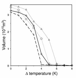
Fig. 39: Inside resolution MIROC Result of the ice sheet model experiment using the result of a warming experiment. The time series of volume change is converted into a sea level, and is expressed. A red line A1B and green line B1 Scenario experiment. A solid line S-fix A dotted line T-fix An experiment (climate in 2100 and afterwards is fixed) blue line is CO2. 4 redoubling experimental findings. Experiment (2300 the climate after a year is fixed) The right figure is a still more long-term change tendency. The following figure is altitude distribution of the stationary solution of each scenario experiment.

The bidirectional joint model which was being developed is employed by the its present location ball simulator. The climate model used the thing incorporating a carbon cycle. An ice sheet model is called in model time one month once, and the surface mass income and outgo which are a boundary condition for an ice sheet are calculated. It becomes the mechanism of calculating an ice sheet flow once a year more, and passing the new geographical feature searched for, ice sheet distribution, and freshwater supply to the ocean to the climate model side. A model is a parallelization model of air 16CPU and sea 16CPU (count 32CPU =4 node), and is the atmosphere. The Greenland ice sheet is contained in one of the CPUs. In about 10 node time product want, the time quadrature for one year takes 2.5 hours, when 4 node employment is carried out. When only the interaction between air-ice sheets is taken into consideration 2100 From a year 2200 Integration to a year is performed and the present result is analyzed.

The border of the Greenland ice sheet is a domain where dissolution is dominant, and it is thought that it has influence to a response with a big change of the amount of dissolution of a there in the case of warming. The amount of dissolution is an element which is strongly influenced to the altitude of an ice sheet depending on temperature as for temperature. Therefore, it is expected that the character of altitude (ice thickness) reappearance of a border has influences of some on an ice sheet response in a warming experiment. Therefore, it can be said that it is important also because of the interpretation of a warming experiment of consideration of how many ice sheet responses are influenced by that the uncertainty of altitude (ice thickness) reappearance of a border is how much and its uncertainty.

The ice sheet model of the former many expresses the time quadrature of ice thickness distribution with a spread type, and is dispelling it numerically. It divides into the method of carrying out difference expression of this spread type greatly, and there are two methods (Hindmarsh and Payne, 1996; Huybrechts et al, 1996). Although any method of reappearance of the inland of an ice sheet is good, it is pointed out that the error of ice thickness reappearance of the border of an ice sheet is large. Moreover, although these two methods become the almost same reappearance inland, reappearance of a border part has a large difference in comparison. Here, the uncertainty of the stationary solution of the Greenland ice sheet resulting from the numeric representation was investigated. Model ice sheets are all. Five Time quadrature was carried out for 10,000 years. Furthermore, in the research using many conventional ice sheet models, a certain mass income-and-outgo model is used for expression of climatic conditions. The mass income-and-outgo model often used is an experiential formula which calculates the amount of dissolution from temperature distribution. Also in the mass income-and-outgo analysis of the ice sheet by GCM, many methods of diagnosing by a mass income-and-outgo model using the temperature distribution of GCM etc. are used. Furthermore, it sees in recent years. The GCM-ice sheet joint model has also introduced the mass income-and-outgo model between them. These are used in order to express the small dissolution region (number 10 km grade) of a space scale with sufficient accuracy. The same method of diagnosing the output of a climate model by a mass income-and-outgo model, and inputting into an ice sheet model also by the ice sheet climate joint model under present employment, is adopted. There was research which compared reproducibility of a mass income-and-outgo model and a heat budget model partly until now (van de Wal 1996; Ohmura 2001). However, there is no research which investigated how the difference in a mass income-and-outgo model would influence the sensitivity of the Greenland ice sheet. In this research, the uncertainty of the stationary solution of the Greenland ice sheet resulting from the difference in a mass income-and-outgo model was investigated using two typical surface mass income-and-outgo models by the same technique as the sensitivity experiment about the above-mentioned numeric representation (under Saito and Abe-Ouchi (inch press), Saito and Abe-Ouchi, and contribution preparation).

One of the surface mass income-and-outgo models used here It is the technique standardly used in the research using (Reeh 1991) and an ice sheet model by the method called Positive Degree Day (PDD). Another It is the technique used by Ohmura et al. (1996), and is the method of estimating the amount of dissolution from summer mean temperature (here, it is henceforth it is referred to as LTI). Although the amount of dissolution by which any technique was observed is often reproduced, when temperature is higher as a feature The amount of dissolution by PDD It is becoming larger than that of LTI.

With four kinds of combination of the ice sheet model considered from a point of the numerical technique and two mass income-and-outgo models, the volume of the stationary solution of the reproduced Greenland ice sheet becomes as it is shown in Fig. 40. It turns out that the uncertainty of the volume of the stationary solution to the same temperature is large in the place where temperature change given especially is high. For example, when the uncertainty of the Greenland ice sheet under the climate which carried out 4K rise in heat uniformly from the present was all dissolved, it became clear that it spread by the solution in which an ice sheet remains from from more than in half. The rise in heat of these 4-5K is included in the sphere of the future warming upsurge predicted from a climate model. That is, it is thought that I hear that uncertainty like this is in the final state of a response of the Greenland ice sheet to global warming of reaching, and it is, and has influence also on presumption of a response of a certain amount of short period of time. Therefore, it can be said that cautions are required for the interpretation of the reproduced ice sheet response enough.

Fig. 40: Volume of Greenland ice sheet stationary solution by difference in numeric representation of equation, and difference in surface mass income-and-outgo model. Thick lines are PDD and a small-gage wire. LTI Result depended on a model. A dotted line and a solid line express the model from which numeric representation is different. A horizontal axis is the temperature distribution of external force.

f. Bibliography

Wild, M. and Ohmura, A. Change in mass balance of polar ice sheets and sea level from high-resolution GCM simulations of greenhouse warming. Ann. Glaciol. 30, 197-203, 2000.

Calanca, P. et al. Gridded temperature and accumulation distributions for Greenland for use in cryospheric models. Ann. Glaciol. 31, 118-120, 2000.

Hindmarsh, R. C. A. and Payne, A. J. Time-step limits for stable solutions of the ice-sheet equation. Ann. Glaciol. 23, 74--85, 1996

Huybrechts, P. et al. The EISMINT benchmarks for testing ice-sheet models. Ann. Glaciol. 23, 1--12, 1996

van de Wal, R. S. W. Mass-balance modelling of the Greenland ice sheet: a comparison of an energy-balance and a degree-day model. Ann. Glaciol. 23, 36--45, 1996. Saito, F. and Abe-Ouchi, A. Sensitivity of Greenland ice sheet simulation to the numerical procedure employed for ice sheet dynamics. Ann. Glaciol. 42, in press.

Ohmura, A. et al. A Possible change in mass balance of Greenland and Antarctic Ice Sheets in the Coming Century. J. Climate 9, 2124--2135, 1996.

Ohmura, A. Physical Basis for the Temperature-Based Melt-Index Method. J. Appl. Meteorol. 40, 753--761, 2001.

Reeh, N. Parameterization of melt rate and surface temperature on the Greenland ice sheet. Polarforschung 59, 113--128, 1991.

g. Research presentation

Paper announcement

Annan,J., J.C.Hargreaves, R.Ohgaito, A.Abe-Ouchi and S.Emori, 2005, Efficiently Constraining Climate Sensitivity with Ensembles of Paleoclimate Simulations. SOLA, Vol.1, 181-184, doi:10.2151/sola. 2005-047.

Jost , A, M.Lunt, M.Kageyama, A.Abe-Ouchi, O.Peyron, P.J.Valdes, and G.Ramstein, 2005, High resolution simulations. Of the last glacial maximum climate over Europe: a solution to discrepancies with continental paleoclimatic reconstructions? Climate Dynamics, DOI 10.1007/s00382-005-0009-4.

Kageyama, M., S.P. Harrison and A. Abe-Ouchi (2005) The depression of tropical snowlines at the Last Glacial Maximum: what can we learn from climate model experiments? Quaternary International, in press.

Kageyama, M., A.Laine, A. Abe-Ouchi and 17 members, 2006, Last Glacial Maximum temperatures over the North Atlantic, Europe and Western Siberia: A comparison between PMIP models, MARGO sea-surface temperatures and pollen-based reconstructions, Quaternary Science Reviews, in press.Saito, F. and A. Abe-Ouchi. (2006) Dependence of simulation and sensitivity of Greenland ice sheet to numerical procedures for ice sheet dynamics. Annals of Glaciology, 42, in press.

Masson-Delmotte, V., M.Kageyama, P.Braconnot, S.Charbit, G.Krinner, C.Ritz, E.Gailyardi, J.Jouzel, A.Abe-Ouchi and 17members, 2005, Past and future polar amplification of climate change: climate model intercomparison and Ice-Core constraints. Climate Dynamics, DOI 10.1007/s00382-005.0081-9.

Saito, F. and A. Abe-Ouchi (2004) Thermal Structure of Dome Fuji and East Queen Maud Land, Antarctica, simulated by a three-dimensional ice sheet model. Annals of Glaciology, 433--438

Saito, F. and Abe-Ouchi, A. Sensitivity of Greenland ice sheet simulation to the numerical procedure employed for ice sheet dynamics. Ann. Glaciol. 42, in press.

Saito. F, A.Abe-Ouchi, H.Blatter, 2006, EISMINT model intercomparison experiments with higher order mechanics. Jounal of Geophysical Research, in press.

Suzuki, T, H. Hasumi, T.T. Sakamoto, T. Nishimura, A. Abe-Ouchi, T. Segawa, N. Okada, A. Oka and S. Emori, 2005, Geophysical Research Letters, 32, L19706, doi:10.1029/2005GL023677

Yamagishi, T., A. Abe-Ouchi, F. Saito, T. Segawa and T. Nishimura (2006) Reevaluation of paleo-accumulation parameterization over northern hemisphere ice sheet during the ice age with a high resolution atmospheric GCM and a 3-D ice sheet model. Annals of Glaciology, 42, in press.