1-2. Oceanic carbon cycle model

a. Summary

The model which included carbon cycle process in the air sea joint general circulation model was developed, and the warming preliminary experiment for investigating the strength of climate-carbon cycle system feedback using it was conducted. It turned out that the strength of such feedback is weak in our model as a result of preliminary experiment. However, much more parameter tuning and firm initialization are required about especially a terrestrial component. There are some which have achieved over other models the results that such feedback is very strong, a result is compared with such a model, and it is necessary to investigate the cause of a difference of feedback intensity. The earth environment frontier research center has participated in international project C4MIP (both carbon cycle-climate joint model comparison project) for performing such activity, and it is expected that an understanding of an earth scale carbon cycle will deepen through an argument there. Distribution of artificial origin CO₂ quantity to be stored by a sea component shows comparatively good coincidence as observation. It can be called desirable result that distribution of artificial origin CO₂ quantity to be stored is often reproduced by warming in view of the purpose of the symbiosis project which placed the focus. Furthermore, the experiment using the model which expressed the seed composition of a plant and a zooplankton explicitly was also conducted, and it investigated about the influence which the climate change of a scale will have on a hydrographic table layer ecosystem for ten years.

b. Research purpose

The total carbonic acid vertical distribution in the ocean is carrying out characteristic distribution to which concentration becomes low near a surface. Such distribution with the big meaning for air sea exchange of carbon dioxide is determined by process, such as a living thing pump alkali pump and a physical pump, and is making contribution with the most important living thing pump resulting from sedimentation which follows the formation and it of an organic matter in a surface ecosystem especially. The efficiency of the living thing pump is influenced by various physical process, such as the depth of a sea mixolimnion, and transportation of the iron by Ekman upwelling and the atmosphere. In order to grasp how much the carbon dioxide discharged by human activities remains in the atmosphere and to make probable prediction of the future carbon dioxide levels in the atmosphere, it is indispensable to model the carbon cycle process in the ocean exactly.

According to the result of the terrestrial-air-sea combined carbon circulation model which a Hadley center (English) and IPSL (France) performed, influence which a climate change has on carbon dioxide absorption of the ocean is made small (Cox et al., 2000; Friedlingstein et al.2001). However, when the result submitted to both the sea carbon cycle model comparison project (Ocean Carbon-Cycle Model Intercomparison Project, OCMIP) is seen, in the sea carbon dioxide absorbed amount future prediction of a baseline performed without taking a climate change into consideration, the variation between models is large and the predicted value in the 2100 time has a twice as many aperture as this between the minimum value and maximum (Fasham, 2003). For prediction of the carbon dioxide levels in the atmosphere, it is required to improve a sea carbon cycle model succeedingly and to reduce such uncertainty. In this subject of research, the simple marine ecosystem model of four variables is included in an oceanic circulation model with a carbon cycle model, the interaction of a sea carbon cycle and a climatic change is investigated, and it aims at developing further and studying construction of a terrestrial-air-sea combined carbon circulation model, and all the ball scale carbon cycles by it.

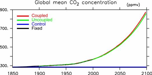
c. A research program, a method, a schedule

the phytoplankton according to Oschlies and Garcon (1999) as an ecosystem model included in an integrated model sea carbon cycle component, nitric acid, a zooplankton, and Deet Wrye -- what added the alteration by Oschlies (2001) to 4 compartment surface ecosystem model of TASS is adopted. Inclusion to the oceanic circulation model of this model was ended even in the 2nd year. Carbon dioxide gradual increase preliminary experiment was conducted in the 3rd more year using the air sea joint model incorporating the above-mentioned sea carbon cycle model and terrestrial carbon cycle model Sim-CYCLE.

In the 4th and afterwards, while conducting continuously experiment which used this joint model, and analysis of a result, it considers building the latest model which cooperated also with the marine research group ("advancement of the carbon cycle model in Pacific Ocean") of the 3rd subject (representation: Toshiyuki Hibiya) of a symbiosis project, and also took the effect of air transportation of iron into consideration. The marine ecosystem model which adopted the iron effect is already developed partly (e. g., Leonard et al., 1999; Archer and Johnson 2000; Moore et al, 2002), and they are considered that it is possible enough to develop our original model to reference. Moreover, about air transportation of iron, it already exists in the form where the dust transportation model which one of research implementation persons developed is immediately included in a general circulation model. The influence which iron transportation according to the atmosphere in the future has on a living thing pump by combining these can be explicitly dealt with now, and coming that it can perform a more concrete argument about the feedback mechanism (Kumar et al.1995; Ridgwell and Watson 2002) through the iron proposed about a glacial-interglacial cycle or global warming etc. is expected.

d. The research program in FY 2004

About the carbon cycle - climate joint model which the prototype has completed, adjustment of details will be finished at an early stage in FY 2004. There are readjustment of biological season parameterization which is needed as an example of details adjustment since the time scales of driving force differ by the terrestrial ecosystem component in a simple substance terrestrial ecosystem model and a joint model, a spin up of a land-and-sea carbon cycle component, etc. Then, the model experiment which put summarizing a result into the view is started.

e. Fruits of work in FY 2004

This section mainly reports the result of the warming preliminary experiment by the model which included terrestrial and a sea carbon cycle model in the air sea joint general circulation model. The same Sim-CYCLE as having used in the III.1-1. paragraph is used for a terrestrial carbon cycle model (Ito and Oikawa, 2002). NPZD4 comparatively easy compartment model by which Oschlies (2001) added improvement to the model of Oschlies and Garcon (1999) at the marine ecosystem model is used. A carbonic acid system chemical process is introduced according to the protocol which both the sea carbon cycle model comparison project (Ocean Carbon Cycle Model Intercomparison Project, OCMIP) recommends to this ecosystem model, and the carbon cycle in the ocean is described. In addition, although the marine ecosystem model existed in FRCGC also before symbiosis project inauguration, this is suitable for seeing the dynamic state of the marine ecosystem itself with complicated structure (Aita et al.2003), and is not adopted in the experiment of this section which put the chief aim on the carbon cycle. However, into this group, the experiment by such a model is also conducted independently and the result is reported to the e.3. paragraph.

The University of Tokyo climate center (CCSR), National Institute for Environmental Studies (NIES), and FRCGC use for an air sea joint general circulation model the inside resolution version of MIROC currently developed together. Since the details of a model are described by Hasumi and Emori (2004), it limits for describing an outline here. The level model resolution by the side of the atmosphere is T42, and this is made into grid size and is equivalent to about 2.8 o. sigma coordinates are adopted as a vertical direction, and 20 layers are taken, making resolution high by the boundary layer near surface of the earth. The model top takes in altitude of about 30km. The horizontal resolution of the direction of longitude by the side of the ocean is 1.4o (= 360/256), and the resolution of the direction of latitude changes spatially. That is, resolution which sets to 1.4o by a side at the equator side very much than 0.56o and 65o, and changes smoothly by the meantime from 8o is adopted. 43 layers were taken in the vertical direction and sigma coordinates and the hybrid coordinate system described by a z coordinate about the other layer are adopted about eight layers near a sea surface. In addition to these 43 layers, a submarine boundary layer exists. Flux regulation is not used when combining the atmosphere and sea both models.

In order to investigate about the strength of the climate-carbon cycle system feedback pointed out by Cox et al. (2000) and Friedlingstein et al. (2001), the preliminary experiment about the global warming by 2100 was conducted. The spin up of a model made the initial value the various places based on climate value data, and performed them for 30 years. Carbon storage and ocean circulation of terrestrial have a long time factor about in 1000, and it can never be said in the spin up for 30 years that it is enough. Moreover, it seems that much more parameter tuning will also be required from now on, and this experiment should be regarded only as a preliminary experiment in the meaning. If experimental findings are investigated, a significant trend actually exists in some variables, such as a soil carbon quantity to be stored. However, before regulation of details is completed, it is important to investigate rough behavior of a model, and the analysis result of a preliminary experiment will be useful also to the interpretation as a result of the full-scale experiment.

Here, three runs are performed. One is a control run, after a spin up fixes CO₂ concentration to 285ppmv, and it runs a model from 1850 to 2100. Other two runs will be called "a joint run" and "an uncombined run." Both of runs give CO₂ concentration observed from 1850 till 1900 to a model, will give CO₂ discharge data (SRES A2) from 1901 till 2100, and will calculate CO₂ concentration inside a model. However, in an uncombined run, CO₂ fixed concentration (it corresponds in 1900) is given to the routine about radiation process, therefore the climate itself does not change. Therefore, the feedback effect of a climate-carbon cycle system is not contained in the uncombined run. On the other hand, by joint run, change of CO₂ concentration calculated using the carbon cycle model is also given to radiation process, and a climatic change breaks out. Since the climatic change which happened here affects a carbon cycle model, the feedback effect of a climate-carbon cycle system is contained in the joint run.

e.2. result and an argument

The time series of global average CO₂ concentration calculated by the model is shown in Fig. 8. It turns out that the model is often reproducing transition of CO₂ concentration by 2000. All over the figure, the green line of a joint run of a red line expresses the result. Although the difference between two experimental findings is small, it turns out that combination of climate and a carbon cycle is committed in the direction to which CO₂ concentration is made to increase. That is, combination of climate and a carbon cycle has the positive feedback effect of accelerating warming. all the balls with which this model predicts this -- since soil temperature and sea surface temperature also rise with the temperature rise called an average of 3.5 oC(s) and the organic matter decomposition in soil is promoted, it is for CO₂ solubility to the ocean to fall. although the effect of the feedback predicted by our model is small -- Cox et al. (2000) The result that there is a bigger feedback effect is obtained in the experiment (especially former) by Friedlingstein et al. (2001). Although it must wait for the experiment which performed details adjustment exactly for this experiment being preliminary as above-mentioned, and obtaining a positive conclusion, arguing about the cause of the difference in a result as compared with other models will lead the result obtained here to a deeper understanding of earth scale carbon cycle process.

Fig. 8: Change of air CO₂ concentration which gave and carried out simulation of source of artificial CO₂ discharge from 1900 to all ball carbon cycles and climate joint model. A dashed line is an observed value, when a red line takes the interaction of warming and a carbon cycle into consideration and a green line does not carry out. The time series of concentration was given to the direct model till 1900. Unit ppmv.

In order to make such a comparative study easy, it is both the carbon cycle-climate joint model comparison project (Coupled Carbon Cycle.). Climate Intercomparison Project and the international project called C4MIP are established. The argument there is to be reflected also in the 4th report of IPCC, and recognizes C4MIP to be an important key to international contributions also as the 2nd subject of symbiosis.

It is necessary to compare between models which are different in the strength of the feedback effect of a climate-carbon cycle system in C4MIP etc. The analysis technique for that is developed by Friedlingstein et al. (2003). By this technique, feedback is divided into four elements and considered. That is, they are four elements of the sensitivity (respectively βAB, βAO) of the carbon cycle of the terrestrial and the ocean to air CO₂ concentration, and the sensitivity (respectively γAB, γAO) of the carbon cycle of the terrestrial and the ocean to temperature change. Below, the outline of this technique is shown. First, the relation between a climatic change and a carbon cycle is linearized, and it expresses as follows.

Here, is after experiment opening CO₂ in the atmosphere increment by a certain time . is the CO₂ emissions of the artificial origin. is CO₂ flux integrated quantity from the atmosphere to the ocean and a terrestrial ecosystem, respectively. is the amount of upsurges of all ball par surface temperature. is surface temperature diversification by factors other than CO₂ (aerosol etc.). If is eliminated from four upper formulas, and it will solve about and will be written as

is obtained.

here and CO₂ in the atmosphere increment in the uncombined run within the limits of which the assumption of linearization consists is expressed. shows the bulk of amplification by feedback. Or it is called usual feedback factor. By investigating the value of , the strength of feedback and the quantitive argument about a factor which brings about feedback are attained.

The result applied to the model of Cox et al. (2000) and Friedlingstein et al. (2001) with the result of having applied this technique to our model is shown in Table 2. Except for βAO, the sensitivity of this experiment is lower than the thing of other two experiments, and, as a result, is a gain factor. g is also lower than the thing of other models. Although such a difference is not clear at present in by what it is brought, the thing with the small (720 or less GtC) carbon quantity to be stored of terrestrial in our model may be related. As Dufresne et al. (2002) pointed out, the CO₂ discharge from soil organic carbon is the important element which forms feedback of a climate-carbon cycle system. Since there is little quantity of soil organic carbon, the CO₂ discharge from there is suppressed, and it is possible that feedback is also small as a result with this experiment. In order to obtain the result which can be equal to a strict argument, the parameter tuning to a terrestrial carbon cycle model which brings about sufficient quantity of a carbon accumulated dose is required. As of March, 2005, such parameter tuning is finished and it will be again about the run for model initial value creation in the middle of calculation.

Table 2: Evaluation of climate-carbon cycle system feedback intensity about three simulations. α Climate sensitivity to CO₂ (K ppmv-1) βAB βAO, Sensitivity to CO₂ in the atmosphere concentration of the carbon cycle of terrestrial and each ocean (GtC ppmv-1) γAB γAO is the sensitivity to the climatic change of the carbon cycle of terrestrial and each ocean. (GtC K-1) g is the gain factor of relative increases of feedback, i.e., the amount of CO₂ in the atmosphere concentration by feedback, and f. It is defined as 1/(1-g).

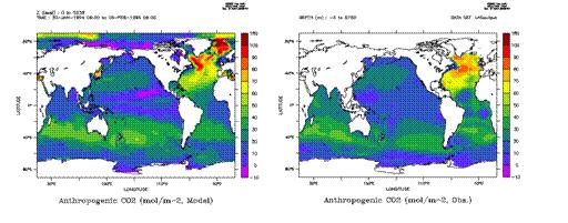
However, according to Dufresne et al. (2002), the rate how much how much is accumulated in vegetation among the carbon cumulative dosage to terrestrial in an uncombined run, and are accumulated in soil about the strength of climate-carbon cycle system feedback has material significance. That is, if carbon accumulated dose increment to vegetation is made to express the thing to ΔVeg and soil as ΔSoi, it will become so strong that feedback is conversely small so that Δ Veg/Δ Soi is large weakly. In the result of this experiment, if ΔVeg and ΔSoi are defined as a difference of the vegetation between a control run and an uncombined run, and the carbon accumulated dose to soil, Δ Veg/Δ Soi will be set to 1.95. This value is larger than what is depended on Cox et al. (2000) (0.54; Dufresne et al, 2002). This value is considered to be the quantity for which it does not depend on the soil carbon accumulated dose of a background greatly, and it is expected that a value also with the comparable experiment after parameter tuning is acquired. Therefore, even if it conducts the same experiment with sufficient carbon accumulated dose through parameter tuning, it is thought that feedback strong in the experiment by a Hadley center does not take place easily.

About the artificial origin CO₂ accumulation in the ocean, the result obtained in this experiment is shown in Fig. 9. With the model result as of 1994, the observational data analysis result by Sabine et al. (2004) is hung up. In northern part North Atlantic Ocean and the Antarctic Ocean in which deep sea water is formed, signs that artificial origin CO₂ accumulated dose is high are known. If it sees on the large-scale scale more than a basin, you say that the model and the observational data analysis result show very good coincidence. It is pointed out by Friedlingstein et al. (2003), Orr et al. and others (2001) that the Antarctic Ocean brings about big uncertainty about an artificial origin CO₂ sea absorbed amount especially. In such ocean space, it can be called very desirable result that the concentration and the distribution pattern of the artificial origin CO 2 show good coincidence. Moreover, about artificial origin CO₂ accumulated dose integrated till 1994, it is 118±19 PgC by evaluation by 108 PgC and Sabine et al. (2004) by the model, and too good coincidence is obtained.

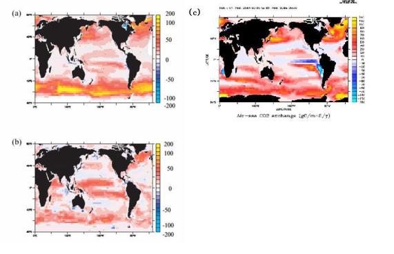
Fig. 9: Artificial origin carbon dioxide distribution in 1994 time accumulated all over the ocean.(Left) A model result, the guess from observation (right) (Sabine et al.2004).Unit molC/m2.

Friedlingstein et al. (2003) is comparing annual average CO₂ flux in the sea surface in the time of CO₂ concentration reaching 700ppmv in an uncombined run about the model of IPSL and a Hadley center. The result of this experiment also shows in Fig. 10 what performed same comparison in addition. It turns out that a big difference is seen between the models of IPSL and Hadley about the Antarctic Ocean which brings about big uncertainty about artificial origin CO₂ sea absorption. The absorbed amount in the Antarctic Ocean as a result of this experiment shows the in-between value of these two models in the Antarctic Ocean. Moreover, in addition to the Antarctic Ocean, in an equatorial region, the offing of Peru, and the offing of Benguela of the Africa east shore, when CO₂ concentration is 700 ppm, in addition, the ocean is emitting CO₂ to the atmosphere, and a characteristic pattern is shown in this experiment. This is in the place where the water mass which becomes the origin of equatorial upwelling or coast upwelling in Peru and the offing of Benguela is shallower than other two models, and is considered because the water mass which upwelling near a sea surface is enabled to go up at the same pace as CO₂ concentration rise in the atmosphere.

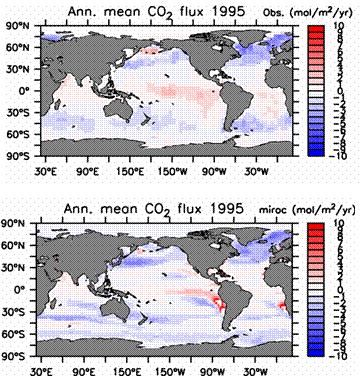
Fig. 10: CO₂ in the atmosphere concentration CO₂ between air-sea surfaces flux in the time of being 700ppmv. A module is gCm-2yr-1 and a color bar is across the board through three panels. A positive value expresses absorption by the ocean. (a) Model of IPSL, (b) Model of Hadley, (c) This experiment.

Moreover, Fig. 11 performed comparison with a model result and observation about CO₂ flux in the sea surface in the present. Since an observation result is standardized to the annual average in 1995, the annual average in 1995 has been shown also about the model result. It turns out that the ocean absorbs CO₂ in a high latitude region, and the model is reproducing the rough feature that discharge strong against an equatorial region exists. However, the burst size in the Peru coast is larger than observation, and the absorption region seen in a model result in a southern Pacific Ocean equatorial region does not exist in observation. As shown in Fig. 8 of a result report in the last fiscal year, the difference with such observation was seen also in the experiment conducted with the oceanographic model simple substance. this report figure 8 -- it depends for existence of such a difference on the place of wind stress so that comparison of b and c may show. Moreover, since the two above-mentioned differences exist in both report figure 8b in Fig. 11 of this paper, and the last fiscal year (FY 2003) and two do not have them in this report figure 8c having become, it can guess making one pair. Also in this experiment, the above-mentioned difference can disappear simultaneously by delicate change of a wind stress field. Since the place where a difference of the Peru coast exists hits coast upwelling域, it can imagine that the strength of wind stress along the shore is an important element. however, the feature like a wind stress field throat must clarify in future analysis about the concrete mechanism which boils whether such differences are brought about and attached.

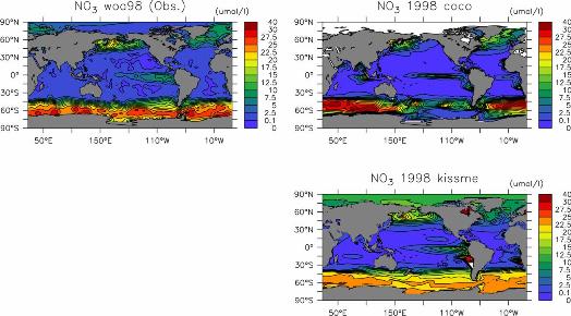
Fig. 11: CO₂ between air-sea surfaces flux as of 1995. A module is gCm-2yr-1. A positive value expresses dishoarding by the ocean. (Above) The observational data based on Takahashi et al. (1999), model (below) result.

Even if the rate that CO₂ absorbed amount by an oceanographic model changes by the case where it does not happen with the case where change of the marine environment accompanying warming takes place is large, it is about 30 percent (IPCC, 2001), and even a possibility that a sink will cross sauce depending on a model is considered that the difference by the model of the feedback intensity of a climate-carbon cycle system is small compared with the case of a certain terrestrial. However, as shown here, about the regional distribution of sea surface CO₂ flux, the difference between models is seen notably. Probably, it needs to be tried hard in the future for reducing the uncertainty resulting from such a difference.

Some comparison with observation is performed also not only about the output directly in connection with CO₂ but about the output from a marine ecosystem model. Fig. 12 shows observation and the model result of surface nitrate concentration. The result depended on the sea simple substance model in the last fiscal year for reference was also shown simultaneously (it is in charge of the experiment A2 of the report table 1 in the last fiscal year). Nitrate concentration is high at an equatorial region and subarctic zone gyre (high latitude ocean space), and it turns out that both the model result is reproducing the feature looked at by observation that it is low at subtropical gyre (inside latitude ocean space). When the result of a sea simple substance model and an integrated model was compared, nitrate concentration was underestimated in the eastern North Pacific of a simple substance model, but in an integrated model, it turns out that the value nearer to observation is acquired. Since the amount of supply of the nutrient salt by Ekman upwelling increased in the integrated model when the place of wind stress changed, it is considered. However, in the result of an integrated model, big overestimation is seen on the Peru coast. It is thought that it corresponds to the excessive dishoarding seen in the figure(Fig. 11) of CO₂ flux in the same station.

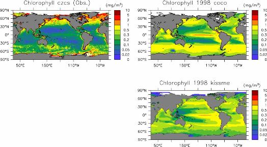
Fig. 12: Surface annual average nitric acid concentration (mmol/m3).(a) Observed value (Conkright et al., 1998), Result of (b) sea simple substance model, Result of (c) integrated model.

In Fig. 13, satellite observation and the model result (the sea simple substance model, integrated model) of surface chlorophyll concentration are compared. The result depended on the sea simple substance model in the last fiscal year for reference was also shown simultaneously. The model is reproducing the tendency for surface chlorophyll concentration to be high in subarctic zone gyre (high latitude region) and an equatorial region, and to be low at subtropical gyre (inside latitude region). However, when figure 13a and c are compared, it turns out that the integrated model has overestimated the surface chlorophyll concentration in an equatorial region and subtropical gyre. Although this tendency is already seen in the experiment by a sea simple substance model, in the result of an integrated model, the width of overestimation is still larger. In the integrated model, the mixolimnion is deeper than the thing of a simple substance model (a figure is not shown), and this is considered because supply of the nutrient salt in subtropical gyre is prosperous. Even if it actually sees Fig. 12, it turns out that nutrient salt concentration is high a little in an integrated model.

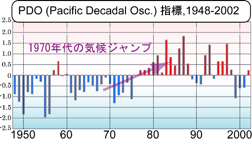
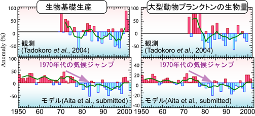
Fig. 13: Surface annual average chlorophyll concentration (mg/m3).(a) Satellite observation by CZCS,
(b) Result of a sea simple substance model, Result of (c) integrated model.

It was slightly complicated so that it might become the reference in the case of the analysis of the result obtained by the "earth system integrated model", but the secular variation numerical simulation was performed by the degree complicated ecosystem model (Intermediate complexity ecosystem model) in the middle of the global three dimension. Although there is little available long-term observational data, the effective range of a model is verifiable by comparing. Specifically, the secular variation of a sea physics place, and the nutrient salt supply by the ocean circulation accompanying the change and change of an ecosystem can be seen by giving the wind stress of the re-analysis data from 1948 of NCEP to 2002, light, sea surface temperature, freshwater flux, etc. to an ecosystem model.

As a climate change of a scale, vibration (PDO) is known well for the Pacific Ocean ten years for tens years, and especially change of the PDO index which happened in the 1970s is called the climate jump or the resume shift (Fig. 14). In the North Pacific, having changed a biological production, and plankton and fish resources is also known with this climate jump.

As for it, the result of the model in the Oyashio region of Japanese waters turns out that change observed mostly is reproduced (Fig. 15). That is, also quantitatively, change of the biological production accompanying the climate jump of the 70s is reproduced. Although change of the large-sized zooplankton used as the food of the fish which is fishing resources is reproduced qualitatively similarly, a little, the range of fluctuation is small compared with observation, and in case it will consider application to fishing resources for the result of this kind of ecosystem model from now on, it needs to consider the cause which produces a difference.

Fig. 14: Time series of Pacific Ocean ten-year change index (Pacific Decadal Oscillation Index, PDO Index).

Fig. 15: Time series of deviation from climate value about living thing (the following figure) primary manufacturing (left-hand side) and large-sized zooplankton (right-hand side) which were reproduced by observation (above figure) and model in Japanese waters Oyashio region.

f. Consideration

f.1. Progress of integrated model development

As seen for the foregoing paragraph, the result of a sea carbon cycle model necessarily shows good coincidence as observation about no points. However, the marine ecosystem model used here is the same as that of that from which it is already used by some other researches also including the value of a parameter, and the result is acquired, and it is a model suitable for using as a standard setup in such a meaning. Moreover, when an example is taken by the purpose of a symbiosis project, the performance most expected from a sea carbon cycle model is simulating the absorbed amount of the artificial origin CO 2 correctly. That artificial origin CO₂ quantity to be stored showed good coincidence as observation in Fig. 9 shows that our model already has sufficient performance at this point. In order to improve coincidence with observation more from now on, it does not consider cleaving the time and the labor of a sea component excessive to parameter tuning. However, since the point that the soil carbon quantity to be stored etc. is not often reproduced about a terrestrial component etc. is directly concerned with the feedback intensity of a climate-carbon cycle system, it is necessary to perform parameter tuning exactly. As above-mentioned, such tuning will be finished as of March, Heisei 17, and the run for initial value creation of a model is performed.

Although it is the stage of preliminary experiment, in case this experiment investigates feedback of a climate-carbon cycle system, it is conducted under the typical setup, and can be called experiment which put paper writing into the view. It can be said that the matter indicated to "d. the research program in FY 2004" was executable.

f.2. Experimental findings using NEMURO

It is due for the change accompanying a climate jump as shown in this paper to take place by what kind of mechanism, and to investigate whether the same mechanism is expressed also by an easy ecosystem from now on so that it may stand, in case the result of the ecosystem in an "earth system integrated model" is analyzed. Although the spatial distribution of the change accompanying the climate jump obtained by the model is harmonic in general, it cannot fully explain it quantitatively to be sea physical environment, fish-resources change, etc. which are observed in each ocean space (for example, movement of the direction of longitude of the front between subtropical-subarctic zone ocean space etc.). By analyzing such reproducibility, it contributes on the certain disposition of future prediction of an "earth system integrated model."

g. Bibliography

Aita, M. N., Y. Yamanaka and M. J. Kishi, Effect of ontogenetic vertical migration of zooplankton on annual primary production ---Using NEMURO embedded in general circulation model---, Fish. Oceanogr., 12, 284-290.

Archer, D. E., and K. Johnson, A model of the iron cycle in the ocean, Global Biogeochem. Cycles, 14, 1436-1446, 2000.

Conkright, M. E., T. D. O'Brien, S. Levitus, T. P. Boyer, C. Stephens, and J. I. Antonov, World Ocean Atlas 1998, NODC, NOAA Atlas NESDIS 12, 1998.

Cox, P. M., R. A. Betts, C. D. Jones, S. A. Spall, and I. J. Totterdell, Acceleration of global warming due to carbon cycle feedbacks in a coupled climate model, Nature, 408, 184-197, 2000.

Dufresene, J.-L., M. Berthelot, L. Bopp, P. Ciais, L. Fairhead, H. Le Treut and P. Monfray, On the magnitude of positive feedback between future climate change and the carbon cycle, Geophys. Res. Lett., 29, doi:10.1029/2001GL013777, 2002.

Fasham, M. J. R. (Ed.), Ocean biogeochemistry: The role of the ocean carbon cycle in global change, IGBP Global Change Series, Springer-Verlag, Berlin Heiderberg New York, 336pp., 2003.

Friedlingstein, P., L. Bopp, P. Ciais, J.-L. Dufrene, L. Fairhead, H. Letreut, P. Monfray, and J. Orr, Positive feedback between future climate change and the carbon cycle, Geophys. Res. Let., 28, 1543-1546, 2001.

Friedlingstein, P., J.-L. Dufresne, P. M. Cox and P. Rayner, How positvie is the feedback between climate change and the carbon cycle- Tellus, 55b, 692-700, 2003.

Hasumi, H, and S. Emori, K-1 coupled GCM (MIROC) description, K-1 Technical Report No.1, Center for Climate System Research, Univ. of Tokyo; National Institute for Envionmental Studies; Frontier Research Center for Global Change, 2004.

IPCC, Climate Change 2001: The scientific basis, Contribution of Working Group I to the Third Assessment Report of the Intergovernmental Panel on Climate Change, Houghton J. T. et al. (eds.), Intergovernmental Panel on Climate Change, Cambridge University Press, Cambridge New York, 2001.

Ito, A., and T. Oikawa, A simulation model of the carbon cycle in land ecosystems (Sim-CYCLE): A description based on dry-matter production theory and plot scale validation, Ecol. Model., 151, 147-179, 2002.

Kumar, N., R. F. Anderson, R. A. Mortlock, P. N. Froelich, P. Kubik, B. Bittrich-Hannen, and M. Suter, Increased biological productivity and export production in the glacial Southern Ocean, Nature, 378, 675-680, 1995.

Leonard, C. L., C. R. McClain, R. Murtugudde, E. E. Hofmann, and L. W. Harding, An iron-based ecosystem model of the central equatorial Pacific, J. Geophys. Res., 104, 1325-1341, 1999.

Moore, J. K., S. C. Doney, D. M. Glover, and I. Y. Fung, Iron cycling and nutrient limitation patterns in surface waters of the World Ocean, Deep-Sea Res. II, 49, 463-507, 2002.

Orr, J. C., E. Maier-Reimer, U. Mikolajewicz, P. Monfray, J. L. Sarmiento, J. R. Toggweiler, N. K. Taylor, J. Palmer, N. Gruber, C. L. Sabine, C. LeQuere, R. M. Key and J. Boutin, Estimates of anthropogenic carbon uptake from four three-dimensional global ocean models, 15, 43-60, 2001.

Oschlies, A., Model-derived estimates of new production: New results point towards lower values, Deep-Sea Res., 48, 2173-2197, 2001.

Oschlies, A. and V. Garcon, An eddy-permitting coupled physical-biological model of the North Atlantic 1. Sensitivity to advection numerics and mixed layer physics, Global Biogeochem. Cycles, 13, 135-160, 1999.

Ridgwell, A. J. and A. J. Watson, Feedback between Aeolian dust, climate, and atmospheric CO₂ in glacial time, Paleoceanography, 17, 1059, doi:10.1029/2001PA000729, 2002.

Sabine, C. L., R. A. Feely, N. Gruber, R. M. Key, K. Lee, J. L. Bullister, R. Wanninkhof, C. S. Wong, D. W. R. Wallace, B. Tilbrook, F. J. Millero, T.-H. Peng, A. Kozyr, T. Ono and A. F. Rios, The oceanic sink for anthropogenic CO₂, Science, 305, 2004.

h. The announcement of a result

Paper publication

Kishi, M. J., T. Okunishi and Y. Yamanaka, Comparing primary production and vertical flux using different ecosystem models in the western North Pacific, J. Oceanogr., 60, 63-73, 2004.

Yamanaka, Y., N. Yoshie, M. Fujii, M. N. Aita and M. J. Kishi, An ecosystem model coupled with nitrogen-silicon-carbon cycles applied to station A-7 in the Northwestern Pacific. J. Oceanogr., 60, 227-241, 2004.

S. L. Smith, Y. Yamanaka and M. J. Kishi, Attempting Consistent Simulations of Stn. ALOHA with a Multi-Element Ecosystem Model. J. Oceanog., 61, 1-26, 2005.

Society announcement

Aita, M.N., and Y.Yamanaka and M.J.Kishi, Interdecadal Variation of the Lower Trophic Ecosystem in the Northern Pacific between 1948 and 2002, 14-in a 3-D implementation of the NEMURO model. October 24 PICES XI Annual Meeting, Honolulu, and 2004.

T. Matsuno, M. Kawamiya, H. Sato and K. Sudo, development of an Integrated Earth System Model on the Earth Simulator, Workshop on Climate Change Research, Oct. 28-29, Yokohama (JAMSTEC, YES), Japan, 2004.

M. Kawamiya, T. Matsuno, and the Kyousei-2 members, Development of an Integrated Earth System Model at FRCGC, Third Japan-EU Workshop on Climate Change Research, Jan. 20-21, Yokohama (JAMSTEC, YES), Japan, 2004.

M. Kawamiya, T. Matsuno, and the Kyousei-2 members, Development of an Integrated Earth System Model at FRCGC, Second International Workshop on the Kyosei Project, Feb. 24-26, Hawaii, U.S, 2004.

Yamanaka, Y., T.Hashioka, M.N.Aita and M.J.Kishi, Ecosystem change in the western North Pacific due to global change obtained by a 3-D ecosystem model.EGU 1st General Assembly, 25-April 30, Nice, and 2004.

Y. Yamanaka, Progress toward high-resolution interannual simulations on the Earth Simulator, and Ocean Carbon-Cycle Model Intercomparison Project - 3 / Northern Ocean-Atmosphere Carbon Exchange Study (NOCES) Second Annual Meeting, 13-May 14, Paris, and 2004.

Michio Kawamiya, Thing - at "the interaction of the atmosphere, water and a living thing, and a climatic change", and the change of the general JAMSTEC lecture meeting "earth environment series" atmosphere and the point of the global warming-Kyoto Protocol, August 4, Tokyo (United Nations University), and 2004.

Development of the earth system integrated model for a Michio Kawamiya, Tomosato Yoshikawa, Taro Matsuno, and earth environment change prediction, the Oceanographic Society of Japan spring convention in FY 2005, 27-March 31, the Tokyo sea university, and 2005.

The possibility of a Michio Kawamiya, Taro Matsuno, and an earth system integrated model, the 52nd time convention of the Ecological Society of Japan, 27-March 30, the Osaka international conference hall, and 2005.