1-3. Dynamic vegetation model

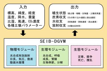
a. Summary

In order to simulate more exactly transitional change of the structure, distribution, and the function of the original vegetation zone of a climatic change which the its present location ball has experienced and which advances quickly, dynamic global vegetation models (DGVMs, Dynamic Global Vegetation Models) called SEIB-DGVM were newly developed. In old trial calculation, SEIB-DGVM was able to reproduce distribution of the vegetation on some phenomena typically observed in a vegetable ecosystem, and the present climatic conditions, or an ecosystem function. After striving for improvement in model reliability by repeating trial calculation and introducing an agro-ecosystem and a land use change module from now on, it is due to make it join together to the earth integrated model to which development is advancing in the 2nd project of symbiosis.

b. Research purpose

Although the structure and the functions (distribution, composition, etc. of a vegetable kind) (the carbon cycle and water cycle) of a vegetable ecosystem are strongly prescribed by climatic environment, the structure and the function of an ecosystem also have feedback-influence on climatic environment through change of the change and the albedo of water loss, a carbon cycle, and land roughness etc. (reviewed by Foley et al.2003). With actualization of global environment problems, the quantitive elucidation is stronger still and an interaction between such climate-vegetation is desired. In order that climatic environment may simulate the influence which it has to the structure and the function of vegetation, the Biogeochemical model of the former many is developed (reviewed by Peng 2000), and those some are treating feedback between climate-vegetation by combining with GCM (General Circulation Model) and both directions (e. g.Woodward et al.1998, Joos et al.2001).

A static model and a dynamic model are large to two, and a Biogeochemical model is classifiable. A static Biogeochemical model (e. g., Neilson 1995, Woodward et al.1995, and Haxeltine & Prentice 1996) simulates physiology process, such as photosynthesis, breathing, and growth, under the inputted climatic environment, and carries out dominance of the vegetation type which makes NPP, LAI, etc. the maximum. The static model assumes that distribution of a vegetable ecosystem reaches a balance immediately to a climatic change in that case. However, even if climate changes in fact, by the time the vegetable ecosystem which was adapted for new environment arises, it will be forecasted that there is an order time delay for several 10 years - thousands of years (Khoyama & Shigesada 1995). Then, in order to simulate exactly transitional change of the original vegetable ecosystem of a climatic change which the its present location ball has experienced and which advances quickly, the dynamic Biogeochemical model has been built (e. g., Foley et al.1996, Friend et al 1997, Sitch et al.2003).

Basic structure is almost common, and any dynamic Biogeochemical model is combining a vegetation dynamic state module (fixing, competition, death, and disturbance being treated) with the existing static model, and enables simulation of the transitional reaction of the vegetation to a climatic change (reviewed by Cramer et al.2001). Although the structure of a dynamic module is various, in order to enable long-term operation in a big geography scale, each has adopted the very simple system. For example, in the LPJ model (Sitch et al.2003), a vegetable kind is represented with ten kinds of Plant Functional Types (following, PFT), and each covering rate of PFT given for every grid is changed according to an amount of growth per each unit area of PFT. In some models, most of the things which are treating competition between PFT(s) in mechanism are representing each PFT with one average individual (An average individual approach), and the competition between individuals in PFT is disregarded.

Then, SEIB-DGVM (Spatialy-Explicit Individual-Base Dynamic-Global-Vegetaion-Model) which has a mechanism vegetation dynamic state module is newly built. SEIB-DGVM sets some representation forests (grassy place) for every grid box, and in it, the arbor treated with the individual base is established, and it grows and dies. The structure of such a model has the following advantages to the conventional dynamic Biogeochemical model. (1) It is expected that competition between the arbor individuals specified according to a local striation affair is expressed appropriately, therefore the speed of the vegetation change accompanying a climate change can be predicted more exactly. (2) The refresh rate of a gap is expressed appropriately and can simulate appropriately change of the carbon balance accompanying such a gap dynamic state. (3) The knowledge of the existing vegetable population dynamics and affinity with data are high, and presumption of a parameter and verification of a model are easy and intuitive. It is shown that analysis is conducted for a long time by the gap model (e. g.Pacala et al.1996), and such a vegetation dynamic state based on local competition can express neither plant succession nor production structure appropriately with a mechanism base nothing to such treatment. However, the gap model was not used by the model of all ball scales for the purpose of reappearance of the forest dynamic state of a specific area until now in many cases. The reason is because requiring more calculation power and more parameters are needed. We conquer these restrictions by developing the vegetation dynamic state module which finished setting up only the dynamic state control mechanism which is common by all vegetable ecosystems only with the easy parameter of acquisition, using the Earth Simulator which has powerful operation power.

c. A research program, a method, a schedule

The basic design of SEIB-DGVM

In order to simulate more exactly transitional change of the structure, distribution, and the function of the original vegetation zone of a climatic change which the its present location ball has experienced and which advances quickly, we developed dynamic global vegetation models (DGVMs, Dynamic Global Vegetation Models) called SEIB-DGVM. This uses the weather and soil data for an input, and outputs both short-term responses (the amount of photosynthesis, respiration rate, etc.) of vegetation, and long-term responses (biomass, distribution of an ecosystem, etc.) (Fig. 16).

Fig. 16: Basic structure and input-output

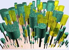
As compared with the conventional DGVMs, that SEIB-DGVM is characterized sets some representation forests (grassy place) for every grid box, the arbor treated with the individual base in it is established, it grows, and it is the point of dying (Fig. 17). For the plant which cannot move from the fixed place, the direction of the next tree withering and light environment being improved rather than some temperature rises, is the reason are a very big environmental change and it adopted this design that a transitional vegetation change cannot be exactly predicted if such an interaction between individuals produced locally is disregarded. Moreover, it also has the advantage that the design of such a model has the knowledge of the existing vegetable population dynamics, and high affinity with data, and presumption of a parameter and verification of a model are easy, and that it is intuitive. Since such approach was accompanied by huge calculation, it became possible for the first time considering employment with an Earth Simulator as a premise.

Fig. 17: Snapshot of virtual stand in SEIB-DGVM (30mx30m temperate mixture lignosa)

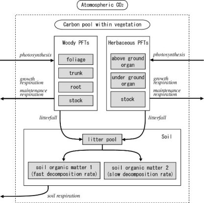
In this model, the land higher plant kind was summarized with a small number of vegetality type (Plant functional types, henceforth, PFTs). This classification is :tropical evergreen broad-leaved tree which assumed the following ten kinds of PFTs, a tropical deciduous broad-leaved tree, a temperate evergreen conifer, a temperate evergreen broad-leaved tree, a temperate deciduous broad-leaved tree, a frigid evergreen conifer, a frigid evergreen broad-leaved tree, a frigid deciduous broad-leaved tree, C3 herb, and C4 herb according to the classification of LPJ-DGVM. Among these, Arbor PFT is treated with an individual base and each arbor individual consists of three parts of a crown, a trunk, and rootlet. Among these, although the crown and the trunk had the form approximated with a pillar, rootlet was expressed only by the biomass. On the other hand, Herb PFT is originally accepted with a leaf, is constituted, and is expressed by the biomass per unit area, respectively.

The flow of the carbon of the whole model is shown in Fig. 18. CO₂ which was air-secondary-twist-picking-crowded and was assimilated by photosynthesis is distributed to each vegetable organ. In connection with the maintenance respiration and growth respiration in each organ, the assimilation products of a certain rate are again emitted into the atmosphere as CO₂. Turnover of each organ, fallen leaves, and the litter generated in connection with the death of an arbor are added to the litter pool in soil. If litter is decomposed, the part will be emitted into the atmosphere as CO₂, and the rest will remain as soil organic carbon. This soil organic carbon is divided into a fraction with a quick decomposition rate, and a late fraction, and these will be emitted into the atmosphere as CO₂, if decomposed.

Fig. 18: Outline of carbon cycle

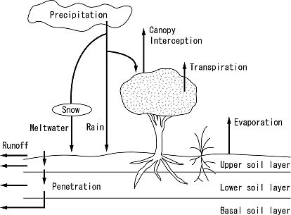
The outline of a water cycle is shown in Fig. 19. At this model, precipitation is the source of supply of the only water, and the supplied water can be stored in a virtual stand with one form of "snow coverage", the "soil upper reservoir water", and "soil lower layer reservoir water." the time of being discharged besides a virtual stand -- "rain interception", "an outflow", "evaporation", and "transpiration" -- one of courses is led. Besides physical environment, such as temperature, a saturation deficit, an amount of insolation, and a soil particle size, the water cycle process of these series receives a curb also from the ecological earmarks, such as a leaf area index and the amount of sunlight composition, strongly, and feedback that the size of soil reservoir water controls a photosynthetic rate commits it.

Fig. 19: Outline of water cycle

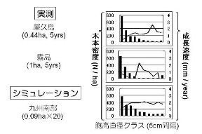
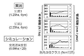
The data set for a simulation

The data set prepared for the model input in Global Soil Wetness Project 2 was used for various soil data. Weather data was used as the daily data for one year by averaging the daily data for ten years in 1990 - 1999 based on The NCEP/NCAR Reanalysis Project (Kistler et al 2001), and used this for the repetition input every year. Soil data was a 1-time grid, and since weather data was supplied by T 62-gauss grid (192x94 points), the data of the land grid which approached most the central point of the grid box which performs a simulation was used as an input value. The initial condition was made into the bare ground where only few herbs exist in all simulations. Moreover, the geographical hetero nature in a grid does not treat in the present version. CO₂ in the atmosphere concentration was fixed as 355 ppm.

d. The research program in FY 2004

dynamic global vegetation model SEIB-DGVM which the rereeling reel completed by the last fiscal year, development is furthered succeedingly and a parameter is adjusted. Moreover, a scale up is performed so that all ball calculation of the conventional model which performs only specific point calculation may be enabled.

e. Fruits of work in FY 2004

Parameter tuning

Some parameters (it is the maximum leaf area per the parameter about the modulus of fixing of Arbor PFT and death and tree crown surface area) about Arbor PFT were adjusted, and the following two distribution was made in agreement between simulation output between actual measurements. (1) Individual frequency distribution for every trunk diameter. (2) The growth rate for every trunk diameter. The ultimate earmark in the dynamic state of a forest and output is reproduced by these. It is because the individual frequency distribution for every trunk diameter reflects the size structure and the existing arbor biomass of a forest and the growth rate for every trunk diameter reflects competition between arbor sizes, and the productivity of a forest directly.

This adjustment was performed for every arbor PFT, and each arbor PFT was performed using the dynamic state data of the stand used as dominant species. In the simulation in adjustment, it was presupposed that only the arbor PFT for adjustment can be established. Moreover, the altitude to input inputted the actual value of the site which obtained each forest dynamic state data. When the annual mean temperature and year precipitation of each site were measured, the data for a model input was processed according to them. namely, That is, it was made the value and uniformity which measured annual mean temperature by adding a steady value to temperature data. Precipitation was made into the value and uniformity which measured year precipitation by applying a quorum value. When annual mean temperature was processed, the same value was added also to soil temperature. An example of the result depended on this adjustment is shown in Figs. 20 and 21. A bar graph shows arbor density and a line graph shows a growth rate.

Fig. 20: Adjustment result of temperate broad leaf evergreen forest

Fig. 21: Adjustment result of frigid needle evergreen forest

Verification about the productivity of a herb

Although SEIB-DGVM is a stage which is continuing adjustment, the result obtained from old trial calculation is introduced to below. These should care about the point which it is provisional and change produces according to future development or progress of parameter tuning.

In a prairie ecosystem, year precipitation specifies vegetable production most strongly and these both relation can revolve by a straight line. If ANPP (g Dry weight / m2-/year) and annual precipitation are set to APPT (mm/year) for above-ground part every year NPP, this regression is on a U.S. central plain. ANPP = -34 + In the prairie of 0.60 APPT and an Asian region ANPP = -30 + 0.59 APPT is presumed (Sala 2001). Both this formula is well alike mutually, and it is known that a big difference will not arise in a tendency between different continents or between herb floras.

Then, it was examined whether this relation could reappear by this model. In two places of Osage (N 36.95, W 96.55) and Central plains (N 40.82, W 104.77), the daily mean precipitation processed constant twice was used for input data, the simulation was performed for 50 years, and, specifically, the relation between every years and year precipitation for the 50th year NPP was obtained. In addition, in this simulation, it assumed that not producing fixing of an arbor and the herb above-ground part NPP were the halves of all the herbs NPP. A result is shown in Fig. 22. Although tendencies, like the direction of a simulation has a remarkable NPP fall when there is little precipitation were also seen, SEIB-DGVM was able to reproduce the actual tendency in production of a prairie ecosystem generally.

Fig. 22: Relation between year precipitation and above-ground part NPP. The plot used the weather data set into which only precipitation was applied and processed by the quorum by the simulation result for 50 years of Central Plaine of a U.S. central plain, and Osage. As for a solid line, a dashed line is a regression line of the survey data in a U.S. central prairie zone in the prairie of an Asian region.

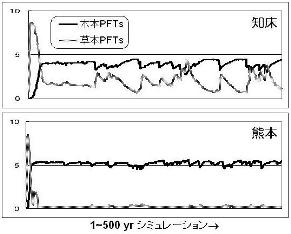
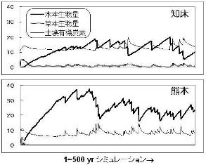
The simulation result in a specific point (arbor PFT)

SEIB-DGVM succeeded in reproducing some phenomena typically observed in plant succession in the simulation in a specific point. Fig. 23 compares diversification of the leaf area index started from the vacant lot in the simulation for 500 years in Shiretoko and Kumamoto (the module repeated m2/m2 and the same climate data every year, and inputted them). . Also in which area, the herb carried out dominance previously, and the changes to which this replaces an arbor gradually have arisen. Moreover, about the period which it takes, Shiretoko which is a cold district was longer. Fig. 24 shows change of the carbon pool in the same simulation (a unit is Kg C/m2). By the time the arbor biomass reached the equilibrium situation in any area, the biomass at the time of taking a long period for a leaf area index to reach a balance and a balance brought the result that Kumamoto which is a warm ground was higher. Moreover, comparison of Figs. 23 and 24 has produced the tendency for a leaf area index to be previously saturated also in which area, and for the biomass to be saturated later than it. These results are fundamentally in agreement with the observation in the outdoors.

Fig. 23: Variation per hour of leaf area index

Fig. 24: Variation per hour of carbon pool

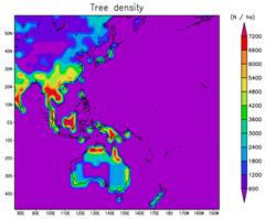
The simulation result in a wide area

The result of the simulation in a larger area is also being obtained. Fig. 25 is distribution of the arbor density of the East Asia and the Oceania area in the 50th year after a simulation start. Signs that a high-density forest develops into the range in which the influence of the monsoon reaches are shown. In fact, although the frigid zone forest existed in the high latitude board of this area, in the model at present, about 50 years of simulation was inadequate for developing a forest into a frigid region.

Fig. 25: Simulation result of arbor density in East Asia and Oceania area. Only the arbor with a breast high diameter of 5cm or more carried out calculation of the result 50 years after starting from a vacant lot. Climate data repeated the same thing every year, and inputted it.

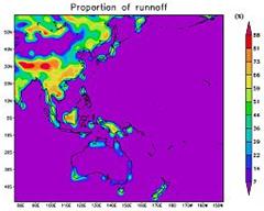
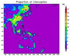
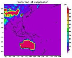
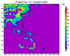
The fundamental action of the water cycle in the same simulation is shown in Figs. 26-29. The rate of a precip that the rate of the precip intercepted evaporates from a soil face most highly (Fig. 27) in the area along the shore where vegetation progresses richly was the highest in the desert of a red centre or the China inland (Fig. 28). The rate of the transpiring precip is the highest at a part for the inland of the high latitude from which the prairie ecosystem developed (Fig. 29), and this area is considered that there is little precipitation and it originates in the high rate of the precip which permeated soil being used for a herb from the first. The outline is in agreement also with the situation where a series of tendencies about these water cycles are actual.

Fig. 26: Rate of precipitation flowing out (annual average)	Fig. 27: Rate of precipitation intercepted (annual average)
Fig. 28: Rate of evaporating precipitation (annual average)	Fig. 29: Rate of transpiring precipitation (annual average)

f. Consideration

A series of simulation results showed clearly that SEIB-DGVM can reproduce the fundamental action and land water cycle of a vegetation dynamic state as an outline. The characteristic design (individual base + explicit space structure) of this model wants to examine what kind of difference is brought to a model output by investigating the change pattern of the ecosystem function at the time of the increase in warming or CO₂ concentration coming, or vegetation distribution, and comparing these with the result of the existing model from now on. And after establishing sufficient reliability, it is due to introduce an agro-ecosystem and a land use change module, and to make it join together during FY 2005 to the earth integrated model to which development is advancing in the 2nd project of symbiosis.

It points out that some problems remain to the last at SEIB-DGVM. Small in all land Tracheophyta to the 1st or it is the point currently summarized by ten kinds of PFTs. For example, in many ecosystems, although the pattern of the changes to a climax arbor kind (wood density is large and a growth rate is slow) from an outrider arbor kind (wood density is small and a growth rate is early) of replacing is seen typically, since SEIB-DGVM defines PFT only supposing a climax arbor kind, recurrence of this pattern cannot be performed. It is the point assumed that the rate of fixing of Arbor PFT is always fixed in the 2nd. Especially in the frigid zone forest, fixing of an arbor is greatly influenced with vegetative propagation ability, seed dormancy nature, shade tolerance, etc. (reviewed by Greene et al.1999), and since the propriety of fixing has specified the vegetation dynamic state strongly, as for such assumption, reappearance of a vegetation dynamic state may be made inaccurate. It is the point of making the 3rd representing a vast area with the small plane space of 30mx30m, and not taking the hetero nature of the scene of a slope etc. into consideration. The correspondence to these problems will serve as a new subject after a joint model is completed.

g. Bibliography

Cramer W. et al, Global response of terrestrial ecosystem structure and function to CO₂ and climate change: results from six dynamic global vegetation models, Global Change Biology, 7, 357-373, 2001.

Foley J. A., An equilibrium model of the terrestrial carbon budget, Tellus, 47B, 310-319, 1995.

Foley J.A., M.H. Costa, C. Delire, N. Ramankutty, and P. Snyder, Green surprise- How terrestrial ecosystems could affect earth's climate, Frontier Ecological Environment, 1, 38-44, 2003.

Friend A.D., A.K. Stevens, R.G. Knox., and M.G.R. Cannell, A process-based, terrestrial biosphere model of ecosystem dynamics (Hybrid v3.0), Ecological Modelling, 95, 249-287, 1997.

Greene D.F., J.C. Zasada, L. Sirois, D.Kneeshaw, H.Morin, I.Charron, and M.-J. Simard. A review of the regeneration dyanmics of North American boreal forest tree species, Can. J. For. Res. 29: 824-839, 1999.

Haxeltine A., I.C. Prentice, and I.D. Cresswell, A coupled carbon and water flux model to predict vegetation structure, Journal of Vegetation Science, 7, 651-666, 1996.

Joos, F., I.C. Prentice, S. Sitch, R. Meyer, G. Hooss, G. Plattner, S. Gerber, and K. Hasselmann, Global warming feedbacks on terrestrial carbon uptake under the Intergovernmental Panel on Climate Change (IPCC) emission scenarios, Global Biogeochemical Cycles, 15, 891-907, 2001.

Kistler R., E. Kalnay., W. Collins, S. Saha, G. White, J. Woollen, M. Chelliah, W. Ebisuzaki, M. Kanamitsu, V. Kousky, van den H. Dool, R. Jenne, and M. Fiorino, The NCEP-NCAR 50-year reanalysis: monthly means CD-ROM and documentation, Bulletin of the American Meteorological Society, 82, 247-267, 2001.

Kohyama, T. and N. Shigesada, A size-distribution-based model of forest dynamics along a latitudinal environmental gradient, Vegetatio, 121, 117-126, 1995.

Neilson R.P., A model for predicting continental-scale vegetation distribution and water balance, Ecological applications, 5, 362-385, 1995.

Pacala, S.W., C.D. Canham, J.A.J. Silander, R.K. Kobe, and E. Ribbens. Forest models defined by field measurements: Estimation, error analysis and dynamics. Ecological Monograph, 66, 1-43, 1996.

Peng C., From static biogeographical model to dynamic global vegetation model: a global perspective on modelling vegetation dynamics, Ecological Modelling, 135, 33-54, 2000.

Sala O.E., Productivity of temperate grassland in Terrestrial Global Productivity, Academic Press, 2001.

Sitch S., B. Smith, I.C. Prentice, A. Arneth, A. Bondeau, W. Cramer, J. Kaplan, S. Levis, W. Lucht, M. Sykes, K. Thonicke, and S. Venevski, Evaluation of ecosystem dynamics, plant geography and terrestrial carbon cycling in the LPJ Dynamic Vegetation Model, Global Change Biology, 9, 161-185, 2003.

Woodward, F.I., T.M. Smith, W.R. Emanuel, A global land primary productivity and phytogeography model, Global Biogeochemical Cycles, 9, 471-490, 1995.

Woodward , F.I., M.R. Lomas, and R.A. Betts, Vegetation-climate feedbacks in a greenhouse world, Phil, Trans. R. Soc. Land. B 353, 29-39, 1998.

h. The announcement of a result

<Oral announcement>

Ecology of a global scale
Akihiko Hisashi Sato and Ito, and Takashi Kohyama
The 52nd Ecological Society of Japan conventions (March, 2005 Osaka)

SEIB-DGVM, a Dynamic Global Vegetation Model for the Kyousei2 project
Hisashi Sato, Akihiko ITOH, Takashi KOHYAMA
The 2nd international workshop on the Kyosei project (February, 2005 Kona, USA)

SEIB-DGVM, a Dynamic Global Vegetation Model for the Kyousei2 project
Hisashi Sato, Akihiko ITOH, Takashi KOHYAMA
Workshop on Climate Change Research (October, 2004 Yokohama)

The terrestrial ecosystem of the future is predicted. -the next generation is dynamic global Vegetation model building-
Akihiko Hisashi Sato and Ito, and Takashi Kohyama
The 51st Ecological Society of Japan conventions (August, 2004 Kushiro)

The terrestrial ecosystem of the future is predicted. -the next generation is dynamic global Vegetation model building-
Akihiko Hisashi Sato and Ito, and Takashi Kohyama
Society of Population Ecology research meeting 2004 (June, 2004 Kyoto, poster announcement)

<Paper publication>

The terrestrial model used by an earth system model: The present condition and the subject of research
Akihiko Ito, Kazuhito Ichii, Katsunori Tanaka, Hisashi Sato、 Seita Emori, Takehisa Oikawa (2004) The weather 51 (4), 227-239.