1-2. Oceanic carbon cycle model

a. Summary

Although the preliminary warming experiment by an air sea combined carbon circulation model was ended in the stage in the last fiscal year, parameter tuning was not fully performed in particular about a terrestrial ecosystem model, but in order to acquire high reliability, some re-experiments needed to be conducted. Parameter tuning and a re-experiment were completed in this fiscal year. As a result of conducting the experiment which investigates the strength of the feedback which the interaction of a climatic change and a carbon cycle brings about to global warming by this model, as for the interaction, it turned out that it works in the direction which raises the carbon dioxide levels in the atmosphere, and has the positive feedback effect of accelerating warming. It is the main cause that disassembly of a soil organic matter is promoted by warming. In this result, the carbon-dioxide-levels differences during the 2 experiments in the 2100 time are 130ppmv. This is converted into surface-of-the-earth mean temperature, and can be called significant quantity in about 1 time. The sensitivity experiment using other parameter sets will also be under execution now in March, Heisei 18. A possibility of a result of being reflected in the 4th report of IPCC with which issue is scheduled for 2007 is high here. Moreover, in the time scale for about several years, although the phenomenon in which it followed in footsteps of change of temperature and CO2 concentration changed was observed, it was checked that the similar phenomenon is reproduced also in a model result. However, the model result of the time lag between temperature change and CO2 concentration change is longer than observation. Moreover, when warming was carried out and analysis detailed about the cause whose CO2 absorbed amount of the ocean decreases was conducted, it turned out that the role with a change of the distribution in the hydrographic table layer of a total carbonic acid and alkalinity significant besides temperature variation is played. Furthermore, the experiment using the model which expressed the seed composition of a plant and a zooplankton explicitly was also conducted, and it investigated about the influence which the climate change of a scale will have on a hydrographic table layer ecosystem for ten years.

b. Research purpose

The total carbonic acid vertical distribution in the ocean is carrying out characteristic distribution to which concentration becomes low near a surface. Such distribution with the big meaning for air sea exchange of carbon dioxide is determined by process, such as a living thing pump alkali pump and a physical pump, and is making contribution with the most important living thing pump resulting from sedimentation which follows the formation and it of an organic matter in a surface ecosystem especially. The efficiency of the living thing pump is influenced by various physical process, such as the depth of a sea mixolimnion, and transportation of the iron by Ekman upwelling and the atmosphere. In order to grasp how much the carbon dioxide discharged by human activities remains in the atmosphere and to make probable prediction of the future carbon dioxide levels in the atmosphere, it is indispensable to model the carbon cycle process in the ocean exactly.

According to the result of the terrestrial-air-sea combined carbon circulation model which a Hadley center (British) and IPSL (France) performed, influence which a climate change has on carbon dioxide absorption of the ocean is made small (Cox et al., 2000; Friedlingstein et al.2001). However, when the result submitted to both the sea carbon cycle model comparison project (Ocean Carbon-Cycle Model Intercomparison Project, OCMIP) is seen, in the sea carbon dioxide absorbed amount future prediction of a baseline performed without taking a climate change into consideration, the variation between models is large and the predicted value in the 2100 time has a twice as many aperture as this between the minimum value and maximum (Fasham, 2003). For prediction of the carbon dioxide levels in the atmosphere, it is required to improve a sea carbon cycle model succeedingly and to reduce such uncertainty. In this subject of research, the simple marine ecosystem model of four variables is included in an oceanic circulation model with a carbon cycle model, the interaction of a sea carbon cycle and a climatic change is investigated, and it aims at developing further and studying construction of a terrestrial-air-sea combined carbon circulation model, and all the ball scale carbon cycles by it.

c. A research program, a method, a schedule

the phytoplankton according to Oschlies and Garcon (1999) as an ecosystem model included in an integrated model sea carbon cycle component, nitric acid, a zooplankton, and Deet Wrye -- what added the alteration by Oschlies (2001) to 4 compartment surface ecosystem model of TASS is adopted. Inclusion to the oceanic circulation model of this model was ended even in the 2nd year. It was shown that conduct a warming experiment using the air sea joint model incorporating the above-mentioned sea carbon cycle model and terrestrial carbon cycle model Sim-CYCLE, and a significant feedback loop will exist between climate and a carbon cycle by 4th more.

Moreover, examination of the latest model development which cooperated also with the University of Tokyo oceanographic institute group ("advancement of the carbon cycle model in Pacific Ocean") of the 3rd subject (delegate: Hibiya Noriyuki) of a symbiosis project, and also took into consideration the cost performance of air transportation of iron was begun in 4th. The marine ecosystem model which adopted the iron effect is already developed partly (e. g., Leonard et al., 1999; Archer and Johnson 2000; Moore et al, 2002), and they are considered that it is possible enough to develop our original model to reference. Moreover, about air transportation of iron, it already exists in the form where the dust transportation model which one of research implementation persons developed is immediately included in a general circulation model. The influence which iron transportation according to the atmosphere in the future has on a living thing pump by combining these can be explicitly dealt with now, and coming that it can perform a more concrete argument about the feedback mechanism (Kumar et al.1995; Ridgwell and Watson 2002) through the iron proposed about a glacial-interglacial cycle or global warming etc. is expected. The 20th century climate reappearance experiment and a warming experiment are due to be conducted in 5th of the last fiscal year using all the ball integrated models that also incorporated atmospheric chemistry process.

d. The research program in the Heisei 17 fiscal year

Parameter tuning of an air sea combined carbon circulation model is completed, the simulation and parameter sensitivity experiment of the carbon cycle at the time of warming are conducted, and a paper is written. Again It participates in C4MIP Phase 1 and activity of 2. After submitting data during the Heisei 16 fiscal year about Phase 1, CO2 concentration seasonal variation etc. analyzes about the phenomenon reproduced in the model. Again The result which requests cooperation from each group who participates about Phase 2, and is related with a sea component is ordered, and a comparative study is performed about the difference in behavior between the oceanographic models about artificial origin carbon dioxide absorption.

e. Fruits of work in the Heisei 17 fiscal year

This year conducted the warming experiment by 2100 using the air oceanic circulation model incorporating carbon cycle process in order to investigate about the strength of the climate and carbon cycle system feedback which were pointed out by Cox et al. (2000) and Friedlingstein (2001). Although the same experiment was conducted also in the last fiscal year, there were problems, like LAI of a high latitude region becomes extremely small for the bias of a climate model. Then, especially this fiscal year experimented by the version improved so that parameter tuning of a terrestrial ecosystem model might fully be performed and a simulation could be performed in an actual more near form.

Since it has already reported in the last fiscal year, it omits, and details of a carbon cycle model or an air sea joint general circulation model are given from the procedure of time quadrature. The spin up of a model fixed CO2 concentration to 285ppmv, made the initial value the various places based on climate value data, and performed them for 280 years. Carbon storage and ocean circulation of terrestrial have a long time factor in 1000 or more, and it can never be said in the spin up in 280 that it is enough. However, it is sufficient period for the grade which removes the time trend of CO2 flux seen immediately after a time quadrature start on all ball scales, and analyzing the result obtained in this experiment has a meaning enough.

Here, three runs are performed. One is a control run, after a spin up fixes CO₂ concentration to 285ppmv, and it runs a model from 1850 to 2100. Other two runs will be called "a joint run" and "an uncombined run." CO₂ discharge data (SRES A2) is given, and CO₂ concentration is calculated inside a model. However, in an uncombined run, CO₂ fixed concentration (285ppmv) is given to the routine about radiation process, and the climate itself does not change. Therefore, the feedback effect of a climate-carbon cycle system is not contained in the uncombined run. On the other hand, by joint run, change of CO₂ concentration calculated using the carbon cycle model is also given to radiation process, and a climatic change breaks out. Since the climatic change which happened here affects a carbon cycle model, the feedback effect of a climate-carbon cycle system is contained in the joint run.

The time series of global average CO2 concentration calculated by the model is shown in Fig. 4. All over the figure, the green line of a joint run of a red line expresses the result. The model is often reproducing transition of CO₂ concentration by 2000. CO2 concentration difference between two runs in the time of 2100 was set to about 130 ppmv(s). This is converted into earth surface mean temperature, and is equivalent to about 1 degree C. Considering that the typical value of warming in the 2100 time which the endowed institution of each country will predict is two to 4 degree C, it can be said that the difference of 1 degree C obtained in this experiment is significant.

Fig. 4: Change of air CO₂ concentration which gave and carried out simulation of source of artificial CO₂ discharge from 1900 to all ball carbon cycles and climate joint model. A dashed line is an observed value, when a red line takes the interaction of warming and a carbon cycle into consideration and a green line does not carry out. Unit ppmv.

Fig. 5 showed the value which pulled the thing of an uncombined run from CO2 concentration in a joint run about the model which has participated in C4MIP as a time series. This figure shows that feedback of the climate-carbon cycle system in our model is comparatively strong in a C4MIP participating model. Friedlingstein et al. (2006) is performing climate-carbon cycle system feedback evaluation of a C4MIP participating model result on the strength based on the technique which Friedlingstein et al. (2003) proposed. According to it, subsequently to the model of a Hadley center, our model has the high response of the terrestrial ecosystem over a climatic change. The thing with strong feedback of our model is the causes with this main in the C4MIP participating model. Moreover, our model is higher than an average also about the factor showing the response of the ocean to a climatic change.

There is big dispersion in the strength of climate-carbon cycle system feedback between models so that it may see in Fig. 5. It is thought that it becomes a good index to see the response of the carbon cycle process over the climate change of a short cycle although it evaluates how realistic the warming result of a C4MIP participating model is. Keeling et al (1989) has actually found out that CO2 concentration also rises with the time delay for about one year, if the time series of CO2 concentration observed in Mauna Roa and all ball mean temperature is compared and all ball mean temperature rises under the influence of El Nino etc. (figure 6a). It is important to investigate whether the phenomenon in which our model is also the same is reproduced, when guessing the actuality of the result shown in Fig. 4.

Fig. 5: Time series of CO2 concentration difference between joint runs and uncombined runs by both climate-carbon cycle joint model comparison project (C4MIP) participating model. A unit is ppmv. A purple solid line with "FRCGC" and notes is our model result. It quotes from Friedlingstein et al. (2006).

The relation between the temperature of a total ball average and CO2 concentration is shown in figure 6b about the period in 1970- 2005 in a model result. In addition, in making this figure, the moving average for 12 more months is given to the data which carried out the total ball average about temperature, and the seasonal variation is removed. The difference of the data which gave the moving average for 12 months about CO2 concentration since a trend was also large over a long period of time, and the data which took the moving average for ten years is taken, and the short cycle ingredient is taken out. It turns out that the model is reproducing the observation result by Keeling et al. (1989) that CO2 concentration fluctuates with a fixed time delay with a rise and descent of temperature. Although this causality is not clear, possibility that it turns out that the soil water content forecast by the land process model MATSIRO as a result of investigating other model output will be changed by a lag for one year, and has the time differential of CO2 concentration and very good correlation from temperature, and elements other than such temperature are related is high. Moreover, the variation of CO2 concentration change in a model result is larger than about 1.5 ppm in figure 6a based on a observation like 2.5 ppm in peak to peak. On the other hand, since the range of fluctuation of temperature is comparable at a model result and observation, it can be said that our model has overestimated the response of the carbon cycle process over the temperature change with the cycle of about several years. However, there is also a place where mechanisms differ by the response of the carbon cycle process in the time scale for about several years, and it to global warming. As an example of the difference in a mechanism, since the temperature rising in Northern Hemisphere high latitude is remarkable in the case of global warming, it can mention that the relative contribution of the response in this latitude belt is higher than the thing in the time scale for about several years etc. Therefore, it cannot necessarily be immediately said from comparison of Fig. 6 that feedback of a climate-carbon cycle system as shown in Fig. 4 is overestimation. However, it is a necessary condition for raising the reliability of prediction to reproduce the phenomenon observed as faithfully as possible. From now on, it strives for improvement in reproducibility by the further parameter tuning and improvement of a model.

Fig. 6: Change CO2 concentration observed in the temperature (solid line) of a total ball average and Mauna Roa by (a) Keeling et al. every year. (b) Change CO2 concentration (green) of the point corresponding to the temperature (red) of the total ball average in a model result, and Mauna Roa every year.

Artificial origin CO2 absorbed amount of the ocean decreases in the former by the case where it does not put in with the case where change of the environment by future warming is taken into consideration as the foregoing paragraph showed. Although it is thought that it is a key factor that the carbon dioxide partial pressure of a hydrographic table layer becomes high by the rise of water temperature as for this, change of the total carbonic acid by change of marine environment and alkalinity etc. is considered as other factors. There are few examples which conducted quantitive analysis about what relative contribution of these many factors has become. In this section, analysis which asks for the relative contribution of many factors mentioned in the top is conducted.

The time series of artificial origin CO2 absorbed amount by the ocean is shown in Fig. 7 about both a joint experiment and an uncombined experiment. Although CO2 in the atmosphere concentration is high, since the carbon dioxide partial pressure (fCO2) of a sea surface is also high simultaneously, the absorbed amount of the ocean does not change the direction of a joint run a lot as a result. In 2070 and afterwards, the effect of sea surface fCO2 rise as shown in Fig. 8 exceeded the effect of the increase in CO2 concentration in the atmosphere, and the direction of artificial origin CO2 absorbed amount in a joint run has decreased a little.

Fig. 7: Artificial origin CO2 absorbed-amount time series by the ocean evaluated by model. black line of a joint run (when the influence of warming is taken into consideration) of a red line expresses the result of an uncombined run (when not putting in).

When Fig. 8 is seen, it turns out in most ocean space except the eastern Pacific Ocean Torrid Zone region that fCO₂ in a joint run is high. Based on an alignment theory, the change of fCO₂ between two runs will be divided according to a factor, and it will argue about it. First, it is considering fCO2 as a function of temperature T, salt S, a total carbonic acid TCO2, and alkalinity Alk,

..... (1)

..... (2)

..... (3)

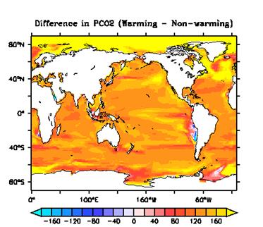
Fig. 8: Difference (ppmv) of carbon dioxide partial pressure (fCO₂) in case (uncombined run) where case (joint run) where reaction of warming is taken into consideration is not considered. The thing in the A.D. 2100 time. When a positive value takes warming into consideration, it is shown that a value becomes high.

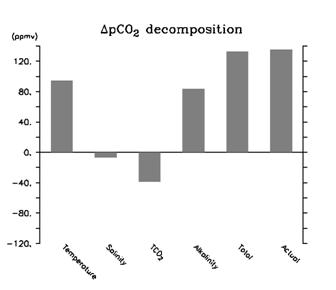
Fig. 9 shows that fCO2 of a joint run is high by the rise of water temperature. However, it turns out that the cost performance that the upsurge of fCO2 by the depression of alkalinity also has comparable contribution, and fCO2 lowers according to the depression of all carbonic acids also has voluntary contribution. He should not catch the rise of fCO2 in a joint run which is seen in Fig. 8 only with the result of a water temperature rise, but should understand it as a result of competition with the effect by the value of a total carbonic acid or alkalinity changing.

In order to investigate how contribution by change of a total carbonic acid and alkalinity which are seen in Fig. 9 is brought about, figure 10a and b showed the geographic distribution of the difference of the total carbonic acid and alkalinity between two runs. It turns out that both distribution is very well alike.

Fig. 9: Result which divided change of fCO₂ between joint run and uncombined run according to factor based on alignment theory, and showed total ball average. Four express change by temperature, salt, a total carbonic acid, and alkalinity from the left, respectively. "Total" shows what "Actual" took the difference of fCO₂ between two runs directly without using alignment approximation, and carried out the total ball average of the sum of change by the factor of the four lefts.

Fig. 10: Difference of (a) total carbonic acid and (b) alkalinity between joint run and uncombined run. A unit is mumol/m3. (c) The difference of the salt between two runs. A unit is PSU. (d) The difference of the (precipitation-amount of evaporation) between two runs. A unit is mm/day. Also in which figure, a positive value shows that a value becomes high in a joint run.

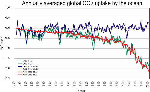
This is the result of being expected to some extent from the biogeochemistry physical process of determining distribution of a total carbonic acid and alkalinity being well (being in a model at least) alike. However, it is interesting that these distribution is very well alike in distribution of the difference of the salt shown in figure 10c here. It turns out that it is what does not depend change of distribution of the total carbonic acid and alkalinity of figure 10a and b on change of a living thing pump, and is depended on change of physical process, such as advective diffusion and precipitation, from this. In case it argues about this kind conventionally especially about change of precipitation, it is not thought as important, but as Dore et al. (2003) pointed out, it may be unable to ignore as a factor which results in change to the amount of air sea CO2 exchange. Change of precipitation was shown in 10d of figures. Although the pattern of the amount distribution of change also has many points which do not resemble the thing of figure 10 a-c, as a value, it can have significant influence on the income and outgo of a total carbonic acid and alkalinity.

It was slightly complicated so that it might become the reference in the case of the analysis of the result obtained by the "earth system integrated model", but the secular variation numerical simulation was performed using the global three dimension middle-scale grade complicated ecosystem model (Intermediate complexity ecosystem model) used comparatively, and the carbon dioxide partial pressure in a sea surface etc. was observed in the Heisei 17 fiscal year. Specifically, the secular variation of a sea physics place, and the nutrient salt supply by the ocean circulation accompanying the change and change of an ecosystem can be seen by giving the wind stress of the re-analysis data from 1948 of NCEP to 2002, light, sea surface temperature, freshwater flux, etc. to an ecosystem model. In order to see the absorbed amount of the carbon dioxide especially by the ocean, the spin up was performed by raising the carbon dioxide partial pressure in the atmosphere according to observation gradually from the 1780s, and repeating beforehand the re-analysis data for 55 years from 1948 to 2002 3 times according to the procedure of the 3rd term of both the international sea carbon cycle model comparative study (Ocean Carbon-cycle Model Intercomparison Project, OCMIP), giving the carbon dioxide partial pressure in the atmosphere from 1760 to 1948.

Fig. 11 is the secular variation of the carbon dioxide absorbed amount by the ocean which carried out the total ball average. The absorbed amount of the artificial origin carbon dioxide by the ocean is increasing gradually as a general trend, and it was come to annual 1.62PgC by the 1980s, and it serves as annual 1.88PgC in the 1990s. In the IPCC Third Assessment Report (2001), it is reported annual 1.9±0.6PgC and annual 1.7±0.5PgC, respectively, and is in agreement within the limits of an error. Moreover, it is the tendency common to many models in OCMIP which the direction of the 1990s is absorbing better than the 1980s. Although the peak whose standard experiment and gradual increase experiment have caused big absorption every 55 years is seen, and this is produced by calculation of a physical place in the South Pole circumference ocean space by large-scale mixture (artificial problem which probably repeats and uses re-analysis data) with the depths, by taking those differences shows being avoided by calculation of the absorbed amount of carbon monoxide at human work.

Fig. 11: Secular variation of carbon dioxide absorbed amount by the ocean which carried out total ball average. The artificial origin carbon dioxide absorbed amount as those differences as a result of calculating by having made it the result (a standard experiment, blue line) of having calculated the carbon dioxide levels in the atmosphere by having made them the value of 278 ppm of the Industrial Revolution, and the observed value (a gradual increase experiment, green line) (red line). Both use the same ocean circulation place, and water temperature and salt distribution. It is that in which the thick line took annual average and the small-gage wire took the moving average for ten years.

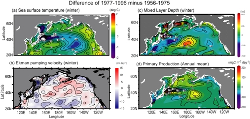
As a climate change of a scale, vibration (PDO) is known well for the Pacific Ocean ten years for tens years, and especially change of the PDO index which happened in the 1970s is called the climate jump or the resume shift (Mantua et al., 1997; figure 12). It was investigated how the sea surface temperature of the North Pacific, mixolimnion depth, a biological production, the amount of planktons, and carbon dioxide partial pressure would change with this climate jump in the Heisei 17 fiscal year. The sea surface temperature of the North Pacific central part fell by 0.4-1.0 degrees C with the climate jump, and rose by 0.2-0.6 degrees C in an east-and-west subtropical zone region or the Gulf of Alaska (on the coast in the Gulf of Alaska, it falls by 0.2-0.6 degrees C). These results are well in agreement with observation of Yasunaka et al. (2002) etc. With the climate jump, Ekman upwelling in subarctic zone ocean space (ocean space consisting mainly of 50N and 180E) is strengthened, and Ekman downwelling is strengthened with subtropical ocean space (ocean space consisting mainly of 30N and 180E). This is because the westerlies in Aleutian low or the Seibu North Pacific were strengthened.

The sea mixolimnion defined by the depth with larger (0.125 kg/m3) density than a sea surface became shallow 10m - 30m, and became deep 20m - 50m in the central North Pacific or western Bering Sea in a western part or the eastern part North Pacific. With change of the above physical place, the basic biological production in the central North Pacific (40N, 180E) corresponding to the increase ocean space of Ekman upwelling increased 30% or more, and decreased about 30% conversely in the mixed water region off Sanriku. In the Gulf of Alaska, although the mixolimnion accompanying a water temperature fall became deep 10m, since Ekman upwelling became weaker, basic biological production became weaker about 20%.

Fig. 12: (a) sea surface temperature before and behind climate jump in the North Pacific, (b) winter mixolimnion depth, (c) Ekman upwelling speed, basic biological production that carried out (d) annual average. The value which subtracted the average before a climate jump (for 20 years from 1956 to 1975) from the average after a climate jump (for 20 years from 1977 to 1996) is shown.

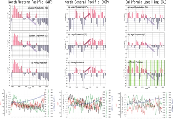
Furthermore, change of each element of the ecosystem in three typical ocean space in the North Pacific and the secular variation of carbon dioxide partial pressure or the carbon dioxide flux between the air-oceans were seen (Fig. 13). In the subtropical ocean space in the western North Pacific (NWP), as Sugimoto & Tadokoro (1998) showed, chlorophyll-a concentration is lower than the 1970s from the 1980s to the first stage of the 1990s. The biomass and the basic biological production of phytoplankton or a zooplankton are low, and our model also depends these on mixolimnion depth's having become shallow with the rise of sea surface temperature and Ekman downwelling having become strong. Between the air-oceans, although carbon monoxide flux is clear, the seasonal variation whose amplitude is comparatively small is shown. Secular variation is small, the change accompanying a climate jump is seldom seen and its correlation with basic biological production is not clear, either.

In the central North Pacific (NCP), when a PDO index is positive, the biomass and the basic biological production of phytoplankton or a zooplankton are increasing. At the point (30N, 160W) where sea surface temperature fell by 0.6 degrees C with strengthening of Aleutian low, and strengthening of westerlies, and the mixolimnion became deep, and the point (35N, 180E) where the mixolimnion became deep although sea surface temperature seldom changed by the advection current effect accompanying the Japan Current way-of-the-world style, although physical mechanisms differ, both increases in supply of the nutrient salt to a hydrographic table layer are raising basic biological production. Carbon monoxide flux shows between the air-oceans the seasonal variation whose amplitude is comparatively large. Furthermore, secular variation is large, the change accompanying a climate jump is also seen, and when basic biological production is high, the result with the large carbon dioxide absorption flux by the ocean is obtained.

In the California upwelling tract (CU), the biomass and the basic biological production of phytoplankton or a zooplankton decrease after a climate jump, and are increasing again late in the 1990s. Coast upwelling in Kaldhol Nia is strongly influenced to ENSO (El Nino south vibration), and the living thing primary manufacturing is decreasing clearly by the penetration of the warm water from south for the year of El Nino (year which carried out the green hatch in Fig. 13). Carbon monoxide flux shows big secular Endo between the air-oceans, and carbon dioxide may not be absorbed from the atmosphere in connection with the penetration of the warm water from south for the year of El Nino, or it may be emitting to the atmosphere.

Fig. 13: The western North Pacific (NWP, left row), the central North Pacific (NCP, central sequence), They are carbon monoxide flux (black line of the lowest figure), and sea surface carbon dioxide partial pressure (blue line of the lowest figure) between the gap (it expresses as percent) from the average of the diatom (from a top) and the biomass of kaiashi in the California upwelling tract (CU, right row), and basic biological production, sea surface temperature (red line of the lowest figure), basic biological production (green line of the lowest figure), and the air-ocean. A yellow-green hatch expresses the El Nino year.

f. Consideration

One of the big targets in the Heisei 17 fiscal year was conducting a warming experiment using the air sea combined carbon circulation model which fully gave parameter tuning, and performing MIP, as a result the contribution to the 4th C4IPCC report. About this point, it can be said that the target was attained enough. Moreover, the paper based on the result shown in this report is also received and published (Kawamiya et al., 2005, Friedlingstein et al., 2006). However, it was not able to attain about the target ("research program in d: Heisei 17 fiscal year" section) "to order the result which requests an affiliation from each group who participates in C4MIP Phase2, and is related with a sea component, and to perform a comparative study about the difference in behavior between the oceanographic models about artificial origin carbon dioxide absorption." Although this performed the presentation request of a result in participating 10 group from us, it is because the group according to presentation had only one. Performing installation of the FTP server for data transfer, simplification of a presentation data format, etc., as for the burden accompanying data presentation, the maximum picking thought that it removed. However, since data presentation requisition from the first was a thing in the middle of a C4MIP proceeding, it is considered to be causality that it was hard to stand the schedule which spares time for data presentation of participating group. I want to consider it as reflection material for our group to play the fixed role in the international community from now on.

g. Bibliography

h. The announcement of a result