1-3 Dynamic vegetation model

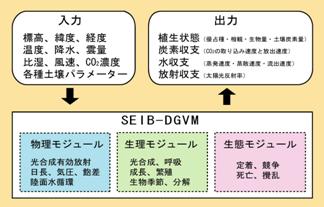
a. Summary

In order to simulate a land ecosystem function in the time factor of thousands of years from hundreds of years, the dynamic global vegetation model (DGVM) which took even the vegetation distribution accompanying a climate change into consideration is needed. After the target of this subgroup develops DGVM uniquely and fully verifies the performance, it is making it combine with an earth integrated model. In the Heisei 17 fiscal year, the performance check was performed with the further improvement of SEIB-DGVM which finished development by the last fiscal year. a until success was carried out to some extent that SEIB-DGVM reproduces some phenomena typically observed in a vegetable ecosystem, and the present vegetation distribution and the ecosystem functional distribution on climatic conditions in old trial calculation.

b. Research purpose

Although the structure and the functions (distribution, composition, etc. of a vegetable kind) (the carbon cycle and water cycle) of a vegetable ecosystem are strongly prescribed by climatic environment, the structure and the function of an ecosystem also have feedback-influence on climatic environment through change of the change and the albedo of water loss, a carbon cycle, and land roughness etc. (Foley et al.2003). With actualization of global environment problems, the quantitive elucidation is stronger still and an interaction between such climate-vegetation is desired. In order that climatic environment may simulate the influence which it has to the structure and the function of vegetation, the Biogeochemical model of the former many is developed (Peng 2000; Arora 2002), and those some are treating feedback between climate-vegetation by combining with GCM (General Circulation Model) and both directions (e. g.Woodward et al., 1998; Cox et al., 2000; Joos et al., 2001).

A static model and a dynamic model are large to two, and a Biogeochemical model is classifiable. A static Biogeochemical model (e. g.Neilson, 1995; Woodward et al., 1995; Haxeltine and Prentice, 1996) simulates physiology process, such as photosynthesis, breathing, and growth, under the inputted climatic environment, and carries out dominance of the vegetation type which makes NPP, LAI, etc. the maximum. The static model assumes that distribution of a vegetable ecosystem reaches a balance immediately to a climatic change in that case. however, even if climate changes in fact, by the time the vegetable ecosystem which was adapted for the new environment arises, it will be forecasted that there will be a time delay of an order from 100 for thousands years (Neilson, 1995; Woodward et al., 1995; Haxeltine and Prentice, 1996).

Then, in order to simulate exactly transitional change of the original vegetable ecosystem of a climatic change which the its present location ball has experienced and which advances quickly, the dynamic Biogeochemical model has been built. A constitution is almost across the board, and any dynamic Biogeochemical model is combining a vegetation dynamic-state module (fixing, emulation, death, and disturbance being treated) with the existing static model, and enables simulation of the transitional reaction of the vegetation to a climatic change (Cramer et al., 2001). Although the structure of a dynamic module is various, in order to enable long-term operation in a big geography scale, each has adopted the very simple system. For example, in the LPJ model (Sitch et al.2003), each covering rate of PFT given for every grid on behalf of a vegetable kind by ten kinds of PFTs (Plant Functional Types) is changed according to NPP per each unit area of PFT. In some models, most of the things which are treating emulation between PFT(s) in frame are representing each PFT with one average individual (An average individual approach), and the emulation between individuals in PFT is disregarded.

The purpose of this research is newly building SEIB-DGVM (Spatialy-Explicit Individual-Base Dynamic-Global-Vegetaion-Model) which has a mechanism vegetation dynamic state module. SEIB sets some representation forests (grassy place) for every grid box, and in it, the arbor treated with the individual base is established, and it grows and dies. The structure of such a model has the following advantages to the conventional dynamic Biogeochemical model. (1) It is expected that competition between the arbor individuals specified according to a local striation affair is expressed appropriately, therefore the speed of the vegetation change accompanying a climate change can be predicted more exactly. (2) The refresh rate of a gap is expressed appropriately and can simulate appropriately change (Shugart, 1998) of the carbon balance accompanying such a gap dynamic state. (3) The knowledge of the existing vegetable population dynamics and affinity with data are high, and presumption of a parameter and verification of a model are easy and intuitive. It is shown that analysis is conducted for a long time by the gap model (Bugmann, 2001), and such a vegetation dynamic state based on local competition can express neither plant succession nor production structure appropriately with a mechanism base nothing to such treatment. However, the gap model was not used by the model of global scales for the purpose of reappearance of the forest dynamic state of a specific area until now in many cases. Since the reason has requiring more calculation power and the tendency to treat a specific interaction to a specific ecosystem, it is because more parameters are needed. We conquered these restrictions by developing the vegetation dynamic state module which it finished setting up only with the easy parameter of acquisition using the newest calculation environment.

c. A research program, a method, a schedule

The basic design of SEIB-DGVM

SEIB-DGVM uses the weather and soil data for an input, and outputs both short-term responses (the amount of photosynthesis, respiration rate, etc.) of vegetation, and long-term responses (biomass, distribution of an ecosystem, etc.) (Fig. 14). As compared with the conventional DGVMs, that SEIB-DGVM is characterized sets some representation forests (grassy place) for every grid box, the arbor treated with the individual base in it is established, it grows, and it is the point of dying (Fig. 15). For the plant which cannot move from the fixed place, the direction of the next tree withering and light environment being improved rather than some temperature rises, is the reason are a very big environmental change and it adopted this design that a transitional vegetation change cannot be exactly predicted if such an interaction between individuals produced locally is disregarded. Moreover, it also has the advantage that the design of such a model has the knowledge of the existing vegetable population dynamics, and high affinity with data, and presumption of a parameter and verification of a model are easy, and that it is intuitive. Since such approach was accompanied by huge calculation, it became possible for the first time considering employment with an Earth Simulator as a premise.

Fig. 14: Basic structure and input-output

Fig. 15: Snapshot of virtual stand in SEIB-DGVM

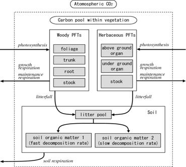
In this model, the land higher plant kind was summarized with a small number of vegetality type (Plant functional types, henceforth, PFTs). This classification is :tropical evergreen broad-leaved tree which assumed the following ten kinds of PFTs(es), a tropical deciduous broad-leaved tree, a temperate evergreen conifer, a temperate evergreen broad-leaved tree, a temperate deciduous broad-leaved tree, a frigid evergreen conifer, a frigid evergreen broad-leaved tree, a frigid deciduous broad-leaved tree, C3 herb, and C4 herb according to the classification of LPJ-DGVM. Among these, Arbor PFT is treated with an individual base and each arbor individual consists of three parts of a crown, a trunk, and rootlet. Among these, although the crown and the trunk had the form approximated with a pillar, rootlet was expressed only by the biomass. On the other hand, Herb PFT is originally accepted with a leaf, is constituted, and is expressed by the biomass per unit area, respectively.

The flow of the carbon of the whole model is shown in Fig. 16. CO₂ which was air-secondary-twist-picking-crowded and was assimilated by photosynthesis is distributed to each vegetable organ. In connection with the maintenance respiration and growth respiration in each organ, the assimilation products of a certain rate are again emitted into the atmosphere as CO₂. Turnover of each organ, fallen leaves, and the litter generated in connection with the death of an arbor are added to the litter pool in soil. If litter is decomposed, the part will be emitted into the atmosphere as CO₂, and the rest will remain as soil organic carbon. This soil organic carbon is divided into a fraction with a quick decomposition rate, and a late fraction, and these will be emitted into the atmosphere as CO₂, if decomposed.

Fig. 16: Outline of carbon cycle

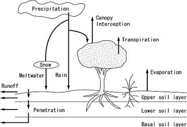
The outline of a water cycle is shown in Fig. 17. At this model, precipitation is the source of supply of the only water, and the supplied water can be stored in a virtual stand with one form of "snow coverage", the "soil upper reservoir water", In case it is discharged besides a virtual forest stand, one course of "a rain blockage", "discharge", "evaporation", and "transpiring" is led. Besides physical environment, such as temperature, a saturation deficit, an amount of insolation, and a soil particle size, the water cycle process of these series receives a curb also from the ecological earmarks, such as a leaf area index and the amount of sunlight composition, strongly, and feedback that the size of soil reservoir water controls a photosynthetic rate commits it.

Fig. 17: Outline of water cycle

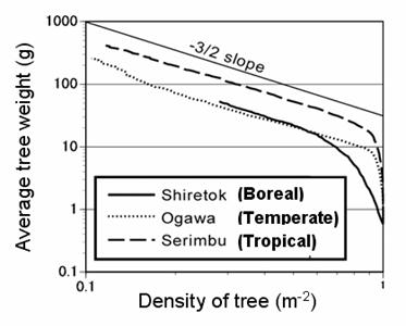
d. The research program in the Heisei 17 fiscal year

The last fiscal year is followed and the Heisei 17 fiscal year is (1). The approvement of SEIB-DGVM, and (2) Evaluation by the various simulations using the present meteorological condition, and (3) It worked considering writing of the paper which releases these results as a center.

e. Fruits of work in the Heisei 17 fiscal year

Verification of 1.5 multiplier law

A small individual usually inclines in the population which exists by high density between the opposite numerical value of a par individual pile, and the opposite numerical value of individual density. - 3/2 of linear relationship is materialized, and this is called -3 / 2 multiplier laws (Yoda et al.1963). The individual pile w is explained to originate in the occupancy area a (namely, the available amount of resources containing light) being proportional to the 2nd power of the vegetable piece l to this phenomenon being proportional to the 3rd power of the vegetable piece l. that is, from and , it is set to and set to . And since the appropriation acreage a of a piece object has the individual density d and the relation of inverse proportion, a relationship called is drawn. Then, in this model, the calculation experiment for confirming whether this relation is materialized was conducted. sapling has been arranged in three areas of the Frigid Zone, the Temperate Zone, and the Torrid Zone by the initial density 1 (tree/m2), respectively, and the simulation for 100 years was performed in them. Fixing of new sapling was not carried out in these 100 years. Fig. 18 is both the logarithm graph that showed change of the relation of the arbor density and the average individual pile in this simulation. After sapling grew to some extent, also in which area, it inclines in general. - Both changed by 3/2 of relations, and the -3-/square-root law was materialized. From this, it can be said that the allometry relation between the monopoly area of trees and the biomass is appropriately reproduced in this model.

Fig. 18: Verification result of -3/2 multiplier law

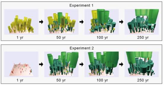
Initial condition dependability to a changes pattern

The greatest special feature of SEIB-DGVM is in the point which simulates the dynamic state of the arbor treated with the individual base in the virtual stand which dealt with space structure clearly. Simulation should be able to do signs that invasion of the arbor which was adapted for new climatic environment is overdue, by the existing arbor's interrupting sunlight in a high-density forest, and continuing occupying a fixing place by this. Then, the reaction of the velocity on the vegetation diversification at the time of an environmental variation was expressed by the difference of the existing vegetation, or the calculation experiment was conducted. A simulation gives the weather data of the Yaku Islands site (20 minutes, north latitude 30-degree annual-mean-temperature ��, the year precipitation of 3200mm, the altitude of 600m, and natural vegetation are temperate evergreen broad-leaved forests), and is a part beam equally about a forest floor point between the arbors PFT which can be established. They are the; processing 1. chill conditions (the temperature and the soil temperature of a yuan lower 10 degrees C than weather data are used) which performed the spin up on two kinds of conditions as follows although the weather data same for a simulation as the time of parameter estimation was used for the input, and processing 2. dryness conditions (precipitation is set to 1/10 from weather data of a yuan). After carrying out the spin up for 1000 years on condition of the above, respectively, the simulation for 250 years was performed.

The physiognomy 250 years 100 years 50 years after a simulation, after a simulation, and after a simulation was shown in Fig. 19 at the simulation start time (at the spin-up completion time) in each processing. Dispensation 1 became the forest in which a temperate needle-leaf tree (TeNE) carries out dominance at the simulation opening time, and two became the temperate grassland in whichCdispensation 3 herb carries out dominance (the herb has not visualized). Although it changed to the forest in which TeBS carries out dominance to a temperate deciduous broad-leaved tree (TeBE) in every dispensation 250 years after the simulation, in dispensation 1, this vegetation diversification was long overdue with the thing with the long tree of TeNE to do for period survival. The difference during such processing was still clearer when time series change of biomass composition was compared. For example, the necessary period until the sum total biomass of TeBE and TeBS reaches 100 Mg C/ha was about 40 years in about 90 years and experiment 2 in the experiment 1, and although the necessary period until it reaches 200 Mg C/ha was about 190 years in the experiment 1, it was about 110 years in the experiment 2. Moreover, in experiment 1, the biomass of TeNE had stopped at the high state about 150 years. It means that the tree with which this was blessed with the ray system affair even when potential vegetation changed with climatic changes can stop for a long time. In addition, the time lag of vegetation change which such an existing arbor brings about is considered to be amplified by restriction of the seed of the arbor which was adapted for new environment (Kohyama & Shigesada 1995), and must be still larger in an actual situation.

Fig. 19: Verification of initial condition dependability of changes pattern

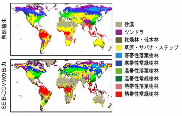
Global experiments

Global simulations were performed by representing each grid of T42 (128x64 points) with one 30mx30m stand. The initial condition was made into the bare ground and the simulation period was carried out 200 years. the fixing conditions of Arbor PFT are as follows. : 50 years of the beginning make the mesh to which sapling can be fixed distribute to all the arbors PFT that can be established in the station equally, and it is made to distribute in proportion to the existing biomass in the 50th and afterwards. Fig. 20 is comparison during the 200-year back of a simulation about distribution and natural vegetation of vegetation. The distribution map of natural vegetation simplified Haxeltine and Prentice (1996). Moreover, the vegetation type standard of classification of a simulation output also used what simplified the standard of Haxeltine and Prentice (1996) (Table 10). In addition, only vegetation data is used for creation of this natural vegetation map, and the output of weather data or other models is not used for it.

On the whole, SEIB-DGVM can say vegetation distribution of global that until succeeded in reappearing to some extent. However, the change of the vegetation type of some areas, especially the vegetation type according to the grade of dryness of a tropical region etc. was not reproduced appropriately. For example, although the tropical vegetation which was adapted for dryness environment, such as a tropical seasonal wood, a savanna, and Xeric woodland, has arisen in natural vegetation, the desert of an output, now stripes is in the India whole region or the south of Sahara in Africa in a simulation.

Fig. 20: Natural vegetation distribution and vegetation distribution which SEIB-DGVM outputted

f. Consideration

A series of simulation results showed clearly that SEIB-DGVM can reproduce the outline of a vegetation dynamic state, a carbon cycle, and a land water cycle at least at some selection points. Moreover, the difference in the existing vegetation was able to express without the special parameterization signs that the migration rate of vegetation was influenced. This is having become possible for the first time by the characteristic design (individual base + explicit space structure) of this model, and is could not accomplish in the conventional DGVMs. The characteristic design of this model wants what kind of to examine further whether it gives to a model output by investigating the change pattern of the ecosystem function at the time of the increase in warming or CO2 concentration coming, or vegetation distribution, and comparing these with the result of the existing model from now on. Moreover, in our research endeavor, a simulation experiment is it due to combine SEIB-DGVM to the earth integrated model KISSME (Kawamiya et al.2005) to which the present development is advanced, and to be conducted what kind of influence the interaction between the land-atmospheres can have on a future earth environment change.

Although SEIB-DGVM is making the vegetation dynamic state mechanism more nearly actual than all the ball vegetation models of the existing throat reflect clearly, it points out that some problems remain. Small in all land Tracheophyta to the 1st or it is the point currently summarized by ten kinds of PFT(s). In global simulations, natural vegetation is considered that one of the reasons which the area which was not able to be reproduced correctly produced has a high possibility of having stemmed from the simplification of this diversity. For example, although xeric woodland/scrub did not arise in this model, it is expected that the shrub kind which turns into dominant species by such a biome is solvable by introducing into a model.

It is the point which sets constant the rate of fixing of the 2nd arbor PFT of a problem. Fixing of an arbor received influence in vegetative propagation ability, seed dormancy nature, shade tolerance, etc. greatly (reviewed by Greene et al.1999), and the propriety of such fixing has specified the vegetation dynamic state and the scene strongly. However, probably the rates of fixing are complicated and various process decided by various factors, and it will not be realistic to take this in with a mechanism base in global models. As one possibility, it is giving the modulus of fixing of each arbor PFT according to a seral stage or each climate zone as the law learned by experience. Starfield & Chapin (1996) has succeeded in reproducing the transitional scene change pattern of Alaska as functions, such as frequency of the elapsed years and the deforestation from climatic conditions and a forest fire, in the model ALFRESCO which used such the law learned by experience as the base.

The 3rd of a problem is the point of representing a vast area with the small plane space of 30mx30m, and not taking the diversity of a scene into consideration. In the model simplified by the conventional altitude, carrying out the parameter rise including the diversity of such a scene is assumed tacitly, and big attention was not paid to this point. However, the relative importance of this problem will also increase as an actual mechanism is made to reflect in a model more strongly. If it is the simulation of a certain limited area, a grid mesh will be simply made fine and it will become essential solution to give an individual environmental condition to each grid mesh. However, for global calculation, in order to save computational complexity, you have to grope for a certain sophisticate(d) technique. This is also a future subject.

Complicating the constitution of a simulation model increases the uncertainty of model output. Therefore, sufficient cautions are required to combine various processes pointed out above one after another. However, in order to predict the phenomenon whose experiment is impossible of predicting the vegetation response at the time of a climate change, in high accuracy, in the phenomenon, you have to introduce an essential process in the form simplified at least. And since the land ecosystem process is complicated and various, it is the enterprise in which it cannot succeed if it does not look for cooperation of many ecologists. SEIB-DGVM can bear a central role in process in which such a terrestrial ecologist's knowledge is made to accumulate. It is because it is all the only ball models that simulate clearly the phenomenon produced with an individual base with SEIB-DGVM being restrained by local space structures, such as fixing, competition, and death of an arbor. Becoming a problem is the point of requiring the calculation power in which SEIB is big.Hurtt et al. (1998) and Moorcroft et al. (2001) have proposed the means of approximating a stochastic demography process, and this makes it possible to treat by the calculation strength to which such a process was restricted. However, if SEIB-DGVM is calculation in one stand, it can fully apply by small workstation, and calculation environment will tend to be substantial increasingly from now on. Furthermore, explicit calculation is suitable for collecting knowledge from the researcher of a broad field from lucid nature and intuition nature being high.

In addition, after striving for improvement in model reliability because SEIB-DGVM adds the further improvement, and introducing an agro-ecosystem and a land use change module, being combined to the earth integrated model to which development is advancing in the 2nd project of symbiosis is planned.

g. Bibliography

Arora, V., 2002. Modeling vegetation as a dynamic component in soil-vegetation-atmosphere transfer schemes and hydrological models. Rev. Geophys. 40, 1006, doi:10.1029/2001RG000103.

Bugmann, H., 2001. A review of forest gap models. Clim. Change 51, 259-305.

Cox, P.M., Betts, R.A., Jones, C.D., Spall, S.A., Totterdell, I.J., 2000. Acceleration of global warming due to carbon-cycle feedbacks in a coupled climate model. Nature 408, 184-187.

Cramer, W., Bondeau, A., Woodward, F.I., Prentice, I.C., Betts, R.A., Brovkin, V., Cox, P.M., Fisher, V., Foley, J.A., Friend, A.D., Kucharik, C., Lomas, M.R., Ramankutty, N., Sitch, S., Smith, B., White, A., Young-Molling, C., 2001. Global response of terrestrial ecosystem structure and function to CO2 and climate change: results from six dynamic global vegetation models. Global Change Biol 7, 357-373.

Foley, J.A., Costa, M.H., Delire, C., Ramankutty, N., Snyder, P., 2003. Green surprise? How terrestrial ecosystems could affect earth's climate. Frontier Ecol. Environ. 1, 38-44.

Greene, D.F., Zasada, J.C., Sirois, L., Kneeshaw, D., Morin, H., Charron, I., Simard, M.-J., 1999. A review of the regeneration dynamics of North American boreal forest tree species. Can. J. For. Res. 29, 824-839.

Haxeltine, A., Prentice, I.C., 1996. BIOME3: An equilibrium terrestrial biosphere model based on ecophysiological constrains, resource availability, and competition among plant functional types. Global Biogeochem. Cycles 10, 693-709.

Hurtt, G.C., Moorcroft, P.R. Pacala, S.W., and Levin, S.A., 1998. Terrestrial models and global change: Challenges for the future. Global Change Biology 4, 581-590.

Joos, F., Prentice, I.C., Sitch, S., Meyer, R., Hooss, G., Plattner, G., Gerber, S., Hasselmann, K., 2001. Global warming feedbacks on terrestrial carbon uptake under the Intergovernmental Panel on Climate Change (IPCC) emission scenarios. Global Biogeochem. Cycles 15, 891-907.

Kawamiya, M., Yoshikawa, C., H. Sato, Sudo, K., Watanabe, S., Matsuno, T., 2005. Development of an Integrated Earth System Model on the Earth Simulator. Journal of Earth Simurator 4, 18-30.

Kohyama, T., Shigesada, N., 1995. A size-distribution-based model of forest dynamics along a latitudinal environmental gradient. Vegetatio 121, 117-126.

Kohyama, T., 2005. Scaling up from shifting-gap mosaic to geographic distribution in the modeling of forest dynamics. Ecol. Res. 20, 305-312.

Moorcroft, P.R., Hurtt, G.C., and Pacala, S.W., 2001. A method for scaling vegetation dynamics: The ecosystem demography model (ED). Ecological Monographs 71, 557-586.

Neilson, R.P., 1995. A model for predicting continental-scale vegetation distribution and water balance. Ecol. Appl. 5, 362-385.

Peng, C.H., 2000. From static biogeographical model to dynamic global vegetation model: a global perspective on modelling vegetation dynamics. Ecol. Modell. 135, 33-54.

Shugart, H.H., 1998. The mosaic theory of natural landscapes. In: Terrestrial ecosystems in changing environments. Cambridge University Press, pp. 178-204.

Sitch, S., Smith, B., Prentice, I.C., Arneth, A., Bondeau, A., Cramer, W., Kaplan, J.O., Levis, S., Lucht, W., Sykes, M.T., Thonicke, K., Venevski, S., 2003. Evaluation of ecosystem dynamics, plant geography and terrestrial carbon cycling in the LPJ dynamic global vegetation model. Global Change Biol. 9, 161-185.

Starfield, A.M., Chapin III, F.S., 1996. Model of transient changes in arctic and boreal vegetation in response to climate and land use change. Ecol. Appl. 6, 842-864.

Woodward, F.I., Lomas, M.R., Betts, R.A., 1998. Vegetation-climate feedbacks in a greenhouse world. Phil. Trans. R. Soc. Land. B 353, 29-39.

Woodward, F.I., Smith, T.M., Emanuel, W.R., 1995. A global land primary productivity and phytogeography model. Global Biogeochem. Cycles 9, 471-490.

Yoda, K., Kira, T., Ogawa, H., Hozumi, K., 1963. Self-thinning in overcrowded pure stands under cultivated and natural conditions (Intraspecific competition among higher plants XI). Journal of Biology, Osaka City University 14, 107-129.

h. The announcement of a result

<Oral announcement>

H. Sato, A. Itoh, and T. Kohyama, SEIB-DGVM: A Spatial-Explicit Individual-Base Dynamic-Global-Vegetation-Model, ESA-INTECOL 2005 joint meeting, Montreal, 2005.

H. Sato, A.Itoh, and T.Kohyama, SEIB-DGVM: A Spatial-Explicit Individual-Base Dynamic-Global-Vegetation-Model, 11 th US-Japan Workshop on Global Change, Yokohama, 2005. (poster)

H. Sato, A.Itoh, and T.Kohyama, SEIB-DGVM: A Spatial-Explicit Individual-Base Dynamic-Global-Vegetation-Model, 11 th US-Japan Workshop on Global Change, Yokohama, 2005. (poster)

H. Sato, A.Itoh, and T.Kohyama, SEIB-DGVM: A Spatial-Explicit Individual-Base Dynamic-Global-Vegetation-Model, 1 st iLEAPS Science Conference, Boulder USA, 2006. (poster)

H. Sato, A. Itoh, and T. Kohyama, SEIB-DGVM: A Spatial-Explicit Individual-Base Dynamic-Global-Vegetation-Model, The 8th International Workshop on Next Generation Climate Models for Advanced High Performance Computing Facilities, Albuquerque USA, 2006.

H. Sato, A. Ito, T. Kohyama: SEIB-DGVM: The status quo and view about a forest ecosystem investigation in A Spatial-Explicit Individual-Base

H. Sato, A. Ito, T. Kohyama: SEIB-DGVM: A Spatial-Explicit Individual-Base Dynamic-Global-Vegetation-Model, a Meteorological Society of Japan 2005 autumn rally, Kobe University, and 2005.

H. Sato, A. Ito, T. Kohyama: SEIB-DGVM: A Spatial-Explicit Individual-Base Dynamic-Global-Vegetation-Model, a Yokohama National University open seminar, Yokohama National University, and 2005.

H. Sato, A. Ito, T. Kohyama: SEIB-DGVM: A Spatial-Explicit Individual-Base Dynamic-Global-Vegetation-Model, the 53rd Ecological Society of Japan rallies, the Niigata convention center, and 2006.

<Paper publication>

H. Sato, A. Itoh, and T. Kohyama, SEIB-DGVM: A New Dynamic Global Vegetation Model using a Spatially Explicit Individual-Based Approach, Submitted to Ecological Modelling.

Kawamiya, M., C. Yoshikawa, H. Sato, K. Sudo, S. Watanabe, and T. Matsuno, Development of an Integrated Earth System Model on the Earth Simulator, Journal of Earth Simurator, 4, 18-30, 2005.