Database for time-series stations K2 and S1

Moored sediment trap data

1. Introduction

In order to verify annual and inter-annual variability of sinking particle fluxes, time-series sediment traps were deployed at several depths at stations K2 and S1. Sediment trap data collected since 2010 are available as one MS Excel file at each station.

Data download

2. Stations, Sampling Periods and Depths

Sediment trap data were obtained from the following stations and time periods.

(1) K2

Three depths (200 m, 500 m, and 4810 m)
Deployment #1 (2010): February 2010–October 2010
Deployment #2 (2010–2011): November 2010–June 2011
Deployment #3 (2011–2012): July 2011–June 2012
Deployment #4 (2012–2013): June 2012–July 2013
Deployment #5 (2013–2014): July 2013–May 2014

(2) S1

Three depths (200 m, 500 m, and 4810 m)
Deployment #1 (2010): February 2010–October 2010
Deployment #2 (2010–2011): November 2010–July 2011
Deployment #3 (2011–2012): July 2011–June 2012
Deployment #4 (2012–2013): July 2012–July 2013
Deployment #5 (2013–2014): July 2013–June 2014

3. Sediment traps

The following time-series sediment traps were used:
200 m: Nichiyu Giken Kogyo SMD26S-26 with 26 collecting cups
500 m, 4810 m: McLane Mark7 series with 21 collecting cups
Before deployment, collecting cups were filled with seawater based 10% buffered formalin as a preservative.

4. Chemical analysis

4.1 Pre-treatment

In the laboratory, sediment trap samples were sieved through 1-mm plastic mesh to eliminate “swimmers”. Samples were then divided into 10 or more fractions by a splitter (McLane splitter). Some fractions were filtered, rinsing with a small amount of distilled water, through pre-weighed Nuclepore filters (0.4-µm pore size) and dried at 50 °C for 24 h. After drying, samples were weighed, and total mass fluxes (TMF: mg m^–2 day^–1) were computed with ancillary data (the number of the fraction, area of the trap mouth (0.5 m²) and sampling period (days)). Subsequently, samples on filters were scraped and pulverized with an agate mortar and stored. Please note that the masses of some samples were too small to scrape from filters. In such cases, after weighing, the Nuclepore filters including the samples were used for ICP-AES measurements (see later). In other cases, a small aliquot of the sample was filtered through a GF/F filter for measurement of particulate carbon and nitrogen.

4.2 Organic carbon, inorganic carbon and nitrogen

For measurement of concentrations of total carbon (TC), samples of approximately 5 mg were precisely weighed in a tin capsule. Samples for measurement of organic carbon (OC) were precisely weighed on GF/F filters. GF/F filters including the samples were placed in a container (plastic Tupperware or desiccator) filled with HCl mist for approximately 24 h to eliminate CaCO₃ (decalcification). After decalcification, filters with samples were wrapped in a tin disk.
Samples in capsules or tin disks were placed in the auto-sampler of an elemental analyzer (Perkin-Elmer 2400) and TC, OC, and the concentration of nitrogen (N) were measured. The instrument was calibrated by using an official certified standard material (acetanilide). Concentrations of inorganic carbon (IC) were determined by the difference between TC and OC. Measurement errors were generally less than 3%. However, if measurement errors were greater than 10%, the calculated IC could be negative for small-volume samples. In this case, IC was estimated from the concentration of calcium (Ca) measured by ICP-AES.

4.3 Trace elements

Concentrations of trace elements were measured by using inductively coupled plasma-atomic emission spectrometry (ICP-AES). For this measurement, samples were decomposed in a nitric acid solution by the fusion method (Huang et al., Limnol. Oceanogr.: Methods 5, 13-22, 2007 and references therein). Samples of approximately 20 mg were precisely weighed in a graphite crucible. Some small samples were collected on Nuclepore filters. In that case, the Nuclepore filter with the sample was placed directly in a graphite crucible. Approximately 140 mg or approximately 7 times the sample volume of lithium metaborate (LiBO₄) was then added and mixed thoroughly with the sample. Samples in graphite crucibles were placed in a muffle kiln (furnace) for 15 minutes at a temperature of 950 °C. Subsequently fused samples were placed in a teflon beaker with approximately 20 ml of a 6% nitric acid solution (HNO₃) and stirred for 1 h. This solution was then filtered through a GF/F filter to eliminate graphite debris, its volume adjusted to 50 ml by addition of 6% HNO₃ solution, and its precise weight determined. Concentrations of trace elements (Si, Ca, Fe, Ti, Mn, Mg, Ba) were measured by ICP-AES (Perkin-Elmer Optima 3300DV). Concentrations of elements were determined by comparison with HNO₃-based ICP-AES standard solutions (Kanto chemicals nos. 20,277–20,280). Rock standards of granite and basalt supplied by the National Institute of Advanced Industrial Science and Technology (formerly the Geological Survey of Japan) (Imai, 2000) were used. These standard solutions were prepared with the same protocol used for sediment trap samples. Measurement errors were less than 5% for every element. However, concentrations of Ti, Mn, and Ba in small-volume samples (usually shallow traps) were sometimes negative (below the detection limit), and there is a large uncertainty associated with these data.

5. Description of data (read me)

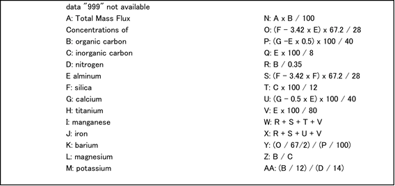
Sediment trap data obtained from each deployment at stations K2 and S1 were compiled.　The following is an explanation of the indicated columns of data.

Contents of the principal columns are as follows:

(1) Data with the designation “999” are not available because no samples were collected or there were no measurements (values under the detection limit).
(2) Column A: Units for total mass flux (TMF) are mg m^–2 day^–1.
(3) Columns B–M: Concentrations of organic carbon (Org-C), inorganic carbon (Inorg-C), nitrogen (N), and trace elements (Al, Si, Ca, Ti, Mn, Fe, Ba, Mg, and K) are in %.
(4) Fluxes of opal, CaCO₃, and lithogenic materials (LM) (mg m^–2 day^–1) were computed as follows:
Column O: Opal flux = (Si – 3.42 x Al) / 100 x 67.2 / 28 x TMF
Column P: CaCO₃ flux = (Ca – 0.5 x Al) / 100 x 100 / 40 x TMF
Column Q: LM flux = Al / 100 x 100 / 8 x TMF
Column R: OM = Org-C / 0.35
(5) Column T: CaCO₃ (Inorg-C based) = Inorg-C x 100 / 12
Column U: CaCO₃ (Ca based) = (Ca – 0.5 x Al) x 100 / 40
(6) Column W (X): Total-I (or Total-II) is the sum of the concentrations of the principal components, that is the sum of the concentrations of OM, Opal, CaCO₃ (Inorg-C based) (or CaCO₃ [Ca based]) and LM. Totals were usually close to 100% (100% ± 10%). However totals for some samples (small-volume samples) were 100% ± 50%.

Note

Details of the sediment trap mooring system are usually described in cruise reports. Please visit the following JAMSTEC MIRAI database site:

6. References

Honda, M. C. (2001) The study of carbon cycle in the western North Pacific by measurement of radiocarbon and sediment trap experiment. Ph.D. thesis, Hokkaido University, 193pp. (in Japanese)
Honda, M. C. et al. (2002) The biological pump in the northwestern North Pacific based on fluxes and major components of particulate matter obtained by sediment-trap experiments (1997-2000). Deep-Sea Research II 49, 5595-5625.