
Publication of the IPCC Sixth Assessment Report (Working Group I) - Scientific Contributions of JAMSTEC Researchers and Their Messages
Emissions of greenhouse gases from human activity chiefly caused global climate change since 1850 and acceleration in the past 30 years – Part II
September 7, 2021

Prabir Patra, Chapter 5 Lead Author
(Earth Surface System Research Center, RIGC, JAMSTEC)
Key points
◆ In the period 1850-1900 and 2010-2019, Concentrations increased from 289.9±3.3 to 398.8±7.3 ppm (38%) for CO2, from 860.4±35.8 to 1829.6±23.9 ppb (113%) for CH4 and from 275.6±2.1 to 327.8±2.9 ppb (19%) for N2O, which lead to cumulative effects on warming of global surface air temperature by 0.79 (range: 0.52–1.25), 0.51 (0.29–0.84) and 0.09 (0.05–0.16) °C, respectively. (Figure SPM.1, Chap 5, Chap 2)
◆ From a physical science perspective, limiting human-induced global warming to a specific level requires limiting cumulative CO2 emissions, along with strong reductions in emissions of other greenhouse gas, e.g., CH4, N2O. Strong, rapid and sustained reductions in CH4 emissions would also limit the warming effect and would improve air quality. (SPM D.1, Chap 6, Chap 5, Chap 3, Chap 4). The faster regrowth (2007-present) of CH4 is driven by emissions from both fossil fuels and agriculture (dominated by livestock) sectors (medium confidence). (Chap 5)
◆Climate model projections show that the uncertainties in atmospheric CO2 concentrations by 2100 are dominated by the differences between emissions scenarios (high confidence). Additional ecosystem responses to warming not yet fully included in climate models, such as CO2 and CH4 fluxes from wetlands, permafrost thaw and wildfires, would further increase concentrations of these gases in the atmosphere (high confidence). (SPM B.4.3, Chap 5)
Effects of well-mixed non-CO2 gases on Global Warming
The non-CO2 species, e.g., methane (CH4), nitrous oxides (N2O), sulfur hexafluoride, chlorofluorocarbons (CFCs, HCFCs, HFCs) are much more powerful greenhouse gases than CO2 per unit mass basis (Chapter 7) and participate in tropospheric and/or stratospheric air chemistry (Chapter 6). Because of their chemical production and loss processes, variability in the atmosphere is a result of the net balance between the sources and sinks on the Earth’s surface and photo-chemical transformation in the atmosphere. Atmospheric transport evens out the regional concentration differences between different parts of the Earth’s atmosphere, depending on lifetimes. A shorter steady-state lifetime of CH4 (9.1±0.9 yr) due to loss in troposphere show much greater space-time variations near the earth’s surface than that for N2O with lifetime of 116±9 yr due to the loss in stratosphere (Chapter 5). Here, detailed discussions around the CH4 and N2O cycling will be covered in this article.
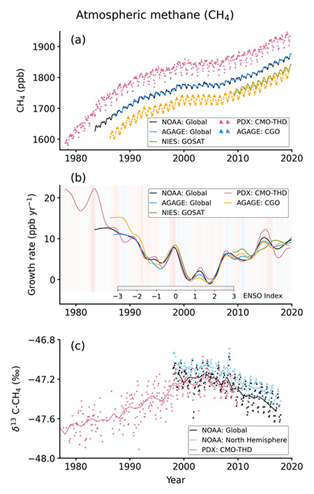
Figure 1: Time series of CH4 concentrations, growth rates and isotopic composition. a) CH4 concentrations, b) CH4 growth rates, c) δ13C-CH4. Data from selected site networks operated by NOAA, AGAGE and PDX (Portland State University). To maintain clarity, data from many other measurement networks are not included here, and all measurements are shown in WMO X2004ACH4 global calibration standard. Global mean values of XCH4 (total-column), retrieved from radiation spectra measured by the greenhouse gases observation satellite (GOSAT) are shown in panels (a) and (b). Cape Grim Observatory (CGO; 41oS, 145oE) and Trinidad Head (THD; 41oN, 124oW) data are taken from the AGAGE network, NOAA global and northern hemispheric (NH) means for δ13C are calculated from 10 and 6 sites, respectively. The PDX data adjusted to NH (period: 1977–2000) are merged with THD (period: 2001–2019) for CH4 concentration and growth rate analysis, and PDX and NOAA NH means of δ13C data are used for joint interpretation of long-term trends analysis. The multivariate ENSO index (MEI) is shown in panel (b). (Figure 5.13)
CH4: Trends, Variability and Budget
Since the start of direct measurements of CH4 in the atmosphere in the 1970s (Figure 1), the highest growth rate was observed during 1977–1986 at 18±4 ppb yr-1 (multi-year mean and 1 standard deviation). This rapid CH4 growth followed the green revolution with increased crop-production and a fast rate of industrialisation that caused rapid increases in CH4 emissions from ruminant animals, rice cultivation, landfills, oil and gas industry and coal mining. The time evolution of δ13C-CH4 suggest the dominance of thermogenic (e.g., oil and gas, coal) and biogenic (e.g., animals, waste) emissions during the periods before and after about 2003.
Methane growth rate has varied widely over the past three decades, and the causes of which have been extensively studied since AR5. The mean growth rate decreased from 15±5 ppb yr-1 in the 1980s to 0.48±3.2 ppb yr-1 during 2000–2006 (the so-called quasi-equilibrium phase) and returned to an average rate of 7.6±2.7 ppb yr-1 in the past decade (2010–2019). Atmospheric CH4 grew faster (9.3±2.4 ppb yr-1) over the last six years (2014–2019) – a period with prolonged El Niño conditions, which contributed to high CH4 growth rates consistent with behaviour during previous El Niño events (Figure 1b). Because of large uncertainties in both the emissions and sinks of CH4, it has been challenging to quantify accurately the methane budget and ascribe reasons for the growth over 1980-2019. To mitigate CH4 emissions, it is critical to understand if the changes in growth rates are caused by emissions from human activities or by natural processes responding to changing climate. If CH4 continues to grow at rates similar to those observed over the past decade, it will contribute to decadal scale climate change and hinder the achievement of the long-term temperature goals of the Paris Agreement.
Figure 2 shows the decadal CH4 budget derived from the Global Carbon Project (GCP)-CH4 synthesis for 1980s, 1990s and 2000s, and for 2010–2017. The imbalance of the sources and sinks estimated by atmospheric inversions (red bars) can be used to explain the changes in CH4 concentration increase rates between the decades. A few studies have debated the role of chemical destruction by OH, the primary sink of methane, in driving changes in the growth of atmospheric methane abundance, in particular after 2006. Studies applying three-dimensional atmospheric inversion, simple multi-species inversion, as well as empirical method using a variety of observational constraints based on OH chemistry, do not find trends in OH large enough to explain the methane changes post-2006. On the contrary, global chemistry-climate models based on fundamental principles of atmospheric chemistry and known emission trends of anthropogenic non-methane SLCFs simulate an increase in OH over this period (see Chapter 6). These contrasting lines of evidence suggest that OH changes may have had a small moderating influence on methane growth since 2007 (low confidence).
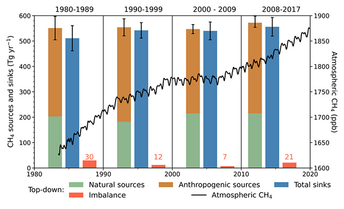
Figure 2: Methane sources and sinks for four decades from atmospheric inversions with the budget imbalance (source-sink; red bars) (plotted on the left y-axis). Top-down analysis of CH4 sources and sinks. The global CH4 concentration seen in the black line (plotted on the right y-axis), representing NOAA observed global monthly mean atmospheric CH4 in dry-air mole fractions for 1983–2019 (Chapter 2, Annex V). Natural sources include emissions from natural wetlands, lakes and rivers, geological sources, wild animals, termites, wildfires, permafrost soils, and oceans. Anthropogenic sources include emissions from enteric fermentation and manure, landfills, waste and wastewater, rice cultivation, coal mining, oil and gas industry, biomass and biofuel burning. The top-down total sink is determined from global mass balance includes chemical losses due to reactions with hydroxyl (OH), atomic chlorine (Cl), and excited atomic oxygen (O1D), and oxidation by bacteria in aerobic soils (Table 5.2). (Cross-Chapter Box 5.2, Figure 1)
Figure 3 shows that modelled wetland emission anomalies for all regions did not exhibit statistically significant trends (high agreement between models, medium evidence). Thus, the inter-decadal difference of total CH4 emissions derived from inversion models and wetland emissions, arises mainly from anthropogenic activities. The timeseries of regional emissions suggest that progress towards atmospheric CH4 quasi-equilibrium was primarily driven by reductions in anthropogenic (fossil fuel exploitation) emissions in Europe, Russia and temperate North America over 1988–2000. In the global totals, emissions equalled loss in the early 2000s. The growth since 2007 is driven by increasing agricultural emissions from East Asia (1997–2017), West Asia (2005–2017), Brazil (1988–2017) and Northern Africa (2005–2017), and fossil fuel exploitations in temperate North America (2010–2017). Evidence from emission inventories at country level and regional scale inverse modelling that CH4 growth rate variability during the 1988 through 2017 is closely linked to anthropogenic activities (medium agreement). Isotopic composition observations and inventory data suggest that concurrent emission changes from both fossil fuels and agriculture are playing roles in the resumed CH4 growth since 2007 (high confidence). Shorter-term decadal variability is predominantly driven by the influence of El Niño Southern Oscillation on emissions from wetlands and biomass burning (Figure 3), and loss due to OH variations (medium confidence), but lacking quantitative contribution from each of the sectors. By synthesising all available information regionally from a-priori (bottom-up) emissions, satellite and surface observations, including isotopic information, and inverse modelling (top-down), the capacity to track and explain changes in and drivers of natural and anthropogenic CH4 regional and global emissions has been improved since the AR5, but fundamental uncertainties related to OH variations remain unchanged.
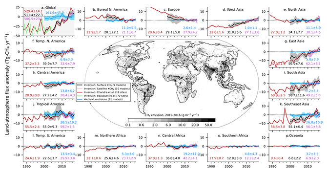
Figure 3: Anomalies in global and regional CH4 emissions for 1988–2017. Map in the centre shows mean CH4 emission for 2010–2016. Multi-model mean (line) and 1-σ standard deviations (shaded) for 2000–2017 are shown for 9 surface CH4 and 10 satellite XCH4 inversions, and 22 wetland models or model variants that participated in GCP-CH4 budget assessment. The results for the period before 2000 are available from two inversions, 1) using 19 sites, and for global totals. The long-term mean values for 2010-2016 (common for all GCP–CH4 inversions), as indicated within each panel separately, is subtracted from the annual-mean time series for the calculation of anomalies for each region. (Cross-Chapter Box 5.2, Figure 2)
N2O: Trends, Variability and Budget
The tropospheric abundance of N2O was 332.1 ± 0.4 ppb in 2019 (Figure 5.15), which is 23% higher than pre-industrial levels of 270.1 ± 6.0 ppb (robust evidence, high agreement). Current estimates are based on atmospheric measurements with high accuracy and density, and pre-industrial estimates are based on multiple ice-core records. The average annual tropospheric growth rate was 0.85 ± 0.03 ppb yr-1 during the period 1995 to 2019 (Figure 4a). The atmospheric growth rate increased by about 20% between the decade of 2000 to 2009 and the most recent decade of 2010 to 2019 (0.95 ± 0.04 ppb yr-1) (robust evidence, high agreement). The growth rate in 2010–2019 was also higher than during 1970–2000 (0.6–0.8 ppb yr-1) and the thirty-year period prior to 2011 (0.73 ± 0.03 ppb yr-1), as reported by AR5. New evidence since AR5 confirms that in the tropics and sub-tropics, large inter-annual variations in the atmospheric growth rate are negatively correlated with the multivariate ENSO index (MEI) and associated anomalies in land and ocean fluxes (Figure 4a).
As assessed by the Special Report on Climate Change and Land (SRCCL), combined firn, ice, air and atmospheric measurements show that the 15N/14N isotope ratio (robust evidence, high agreement) as well as the predominant position of the 15N atom in atmospheric N2O (limited evidence, low agreement) has changed since 1940 (Figure 4b,c) whereas they were relatively constant in the pre-industrial period, suggesting that the isotopically light N2O was emitted from anthropogenic sources, such as the agricultural soil and industry.
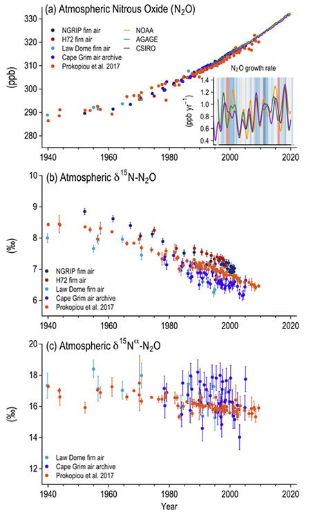
Figure 4. Changes in atmospheric N2O and its isotopic composition since 1940. (a) Atmospheric N2O abundance (parts per billion, ppb) and growth rate (ppb yr-1), (b) δ15N of atmospheric N2O, and (c) alpha-site 15N–N2O. Estimate are based on direct atmospheric measurements in the AGAGE, CSIRO, and NOAA networks, archived air samples from Cape Grim, Australia, and firn air from NGRIP Greenland and H72 Antarctica, Law Dome Antarctica, as well as a collection of firn ice samples from Greenland. Shading in (a) is based on the multivariate ENSO index, with red indicating El Niño conditions. (Figure 5.15)
The synthesis of bottom-up estimates of N2O sources (Figure 5) yields a global source of 17.0 (12.2–23.5) TgN yr-1 for the years 2007–2016. This estimate is comparable to AR5, but the uncertainty range has been reduced primarily due to improved estimates of ocean and anthropogenic N2O sources. Since AR5, improved capacity to estimate N2O sources from atmospheric N2O measurements by inverting models of atmospheric transport provides a new and independent constraint for the global N2O budget. The decadal mean source derived from these inversions is remarkably consistent with the bottom-up global N2O budget for the same period, however, the split between land and ocean sources based on atmospheric inversions is less well constrained, yielding a smaller land source of 11.3 (10.2–13.2) TgN yr-1 and a larger ocean source of 5.7 (3.4–7.2) TgN yr-1, respectively, compared to bottom-up estimates.
Supported by multiple studies and extensive observational evidence (Figure 5), anthropogenic emissions contributed about 40% (7.3; uncertainty range: 4.2–11.4 TgN yr-1) to the total N2O source in 2007–2016 (high confidence). This estimate is larger than in AR5 (WGI, 6.4.3) due to a larger estimated effect of N deposition on soil N2O emission and the explicit consideration of the role of anthropogenic N in determining inland water and estuary emissions. Based on bottom-up estimates, anthropogenic emissions from agricultural nitrogen use, industry and other indirect effects have increased by 1.7 (1.0–2.7) TgN yr-1 between the decades 1980–1989 and 2007–2016, and are the primary cause of the increase in the total N2O source (high confidence). Atmospheric inversions indicate that changes in surface emissions rather than in the atmospheric transport or sink of N2O are the cause for the increased atmospheric growth rate of N2O (robust evidence, high agreement). However, the increase of 1.6 (1.4–1.7) TgN yr-1 in global emissions between 2000–2005 and 2010–2015 based on atmospheric inversions is somewhat larger than bottom-up estimates over the same period, primarily because of differences in the estimates of land-based emissions, since the global budget of N2O is well constrained by atmospheric data and global ocean emission is not expected to change rapidly either by the bottom-up or inversion estimates.
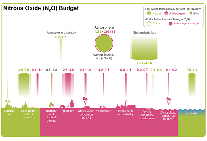
Figure 5: Global nitrous oxide (N2O) budget (2007–2016). Values and data sources as in Table 5.3. The atmospheric stock is calculated from mean N2O concentration, multiplying a factor of 4.79 ± 0.05 Tg ppb-1. Pool sizes for the other reservoirs are largely unknown. (Figure 5.17)
Relative Importance of regional CO2, CH4 and N2O emissions
The total influence of anthropogenic greenhouse gases (GHGs) on the Earth’s radiative balance is driven by the combined effect of those gases (Topics 1, Figure 1). This section compares the balance of the sources and sinks of these three gases and their regional net flux contributions to the radiative forcing. CO2 has multiple residence times in the atmosphere from one year to many thousands of years, and N2O has a mean lifetime of 116 years. They are both long-lived GHGs, while CH4 has a lifetime of 9.1 years and is considered a short-lived GHGs. Owing to the shorter lifetime of CH4, the effect of reduction in emission increase rate on the ERF increase is evident at inter-decadal timescales.
Atmospheric abundance of GHGs is proportional to their emissions-loss budgets in the Earth’s environment. There are multiple metrics to evaluate the relative importance of different GHGs for the global atmospheric radiation budget and the socioeconomic impacts. Metrics for weighting emissions are further developed in the AR6 of IPCC WG-III and WG-I (AR6 Chapter 7). Here, (Figure 6 shows the regional emissions of the three main GHGs. The economically developed regions of East Asia, Europe, Temperate North America and West Asia, the net CO2 fluxes dominates the rest of the world (high confidence) (Figure 6). East Asia, South Asia, Southeast Asia, Tropical South America, Temperate North America and Central Africa are the dominant sources of current CH4 fluxes (Figure 6). The N2O emissions are dominated by the regions of intense agriculture involving nitrogen fertilisers. Only boreal North America showed total net sinks of CO2, while close to flux neutrality is observed for North Asia, Southern Africa, and Australasia. Persistent emission of CO2 is observed for Tropical and South America, northern Africa, and southeast Asia (medium confidence). The medium confidence arises from large uncertainties in the estimated non-fossil fuel CO2 fluxes over these regions due to the lack of high-quality atmospheric measurements.
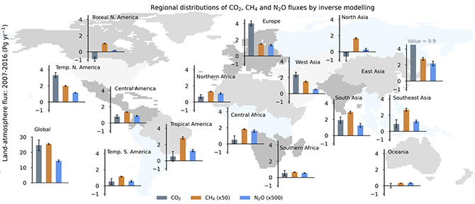
Figure 6: Regional distributions of net fluxes of CO2, CH4 and N2O on the Earth’s surface (Full Molar Mass). The region divisions, shown as the shaded map, are made based on ecoclimatic characteristics of the land. The fluxes include those from anthropogenic activities and natural causes that result from responses to anthropogenic GHGs and climate forcing (feedbacks). The CH4 and N2O emissions are weighted by arbitrary factors of 50 and 500, respectively, for depiction by common y-axes. Fluxes are shown as the mean of the inverse models as available from. (Figure 5.19)

◆Further reading:
- 1)
- モデル解析を基にした温室効果気体の全球規模循環に関する研究 -2016年度堀内賞受賞記念講演- (Study of the global cycle of greenhouse gases using atmospheric chemistry-transport model)
https://www.metsoc.jp/tenki/english/TENKI_e-index17.html - 2)
- China's Carbon Dioxide (CO2) Emissions Have Been Overestimated - Advancement in verification of fossil fuel CO2 and CH4 sources from China -
http://www.jamstec.go.jp/e/about/press_release/20170516_2/ - 3)
- 過去30年間のメタンの大気中濃度と放出量の変化 〜化石燃料採掘と畜産業による人間活動が増加の原因に〜
https://www.jamstec.go.jp/j/about/press_release/20210129/ - 4)
- 大気観測が捉えた新型ウイルスによる中国の二酸化炭素放出量の減少 ~波照間島で観測されたCO2とCH4の変動比の解析~
http://www.jamstec.go.jp/j/about/press_release/20201105/ - 5)
- 世界のメタン放出量は過去20年間に10%近く増加主要発生源は、農業及び廃棄物管理、化石燃料の生産と消費に関する部門の人間活動
https://www.jamstec.go.jp/j/about/press_release/20200806/ - 6)
- 世界の一酸化二窒素(N2O)収支 2020年版を公開
http://www.jamstec.go.jp/j/about/press_release/20201008_2/ - 7)
- Nitrogen fertilisers are incredibly efficient, but they make climate change a lot worse
https://theconversation.com/nitrogen-fertilisers-are-incredibly-efficient-but-they-make-climate-change-a-lot-worse-127103
◆IPCC AR6 WGI報告書出典:
Full report
IPCC, 2021: Climate Change 2021: The Physical Science Basis. Contribution of Working Group I to the Sixth Assessment Report of the Intergovernmental Panel on Climate Change [Masson-Delmotte, V., P. Zhai, A. Pirani, S. L. Connors, C. Péan, S. Berger, N. Caud, Y. Chen, L. Goldfarb, M. I. Gomis, M. Huang, K. Leitzell, E. Lonnoy, J. B. R. Matthews, T. K. Maycock, T. Waterfield, O. Yelekçi, R. Yu and B. Zhou (eds.)]. Cambridge University Press. In Press.
AR6 Climate Change 2021: The Physical Science Basis(外部リンク)
Summary for Policymakers
IPCC, 2021: Summary for Policymakers. In: Climate Change 2021: The Physical Science Basis. Contribution of Working Group I to the Sixth Assessment Report of the Intergovernmental Panel on Climate Change [Masson-Delmotte, V., P. Zhai, A. Pirani, S. L. Connors, C. Péan, S. Berger, N. Caud, Y. Chen, L. Goldfarb, M. I. Gomis, M. Huang, K. Leitzell, E. Lonnoy, J. B. R. Matthews, T. K. Maycock, T. Waterfield, O. Yelekçi, R. Yu and B. Zhou (eds.)]. Cambridge University Press. In Press.
Chapter 5
Josep G. Canadell, J. G., P. M.S. Monteiro, M. H. Costa, L. Cotrim da Cunha, P. M. Cox, A. V. Eliseev, S. Henson, M. Ishii, S. Jaccard, C. Koven, A. Lohila, P. K. Patra, S. Piao, J. Rogelj, S. Syampungani, S. Zaehle, K. Zickfeld, 2021, Global Carbon and other Biogeochemical Cycles and Feedbacks. In: Climate Change 2021: The Physical Science Basis. Contribution of Working Group I to the Sixth Assessment Report of the Intergovernmental Panel on Climate Change [Masson-Delmotte, V., P. Zhai, A. Pirani, S. L. Connors, C. Péan, S. Berger, N. Caud, Y. Chen, L. Goldfarb, M. I. Gomis, M. Huang, K. Leitzell, E. Lonnoy, J. B. R. Matthews, T. K. Maycock, T. Waterfield, O. Yelekçi, R. Yu and B. Zhou (eds.)]. Cambridge University Press. In Press.