
Before you know it it’s fall and the leaves are starting to change color (along with the Climate Watch banner). With the oppressive summer heat gone, it’s the perfect time to do outdoor sports or enjoy the foods that fall has to offer. Among those, the Pacific saury (サンマ or sanma in Japanese) is particularly popular in Japan. You can see a depiction of this prized fish in the Climate Watch banner. On the downside, this is also the beginning of the cold and flu season, so please stay warm.
This post is the second edition of our forecast verification (see here for the first one), and will examine the quality of the prediction for this year’s summer.
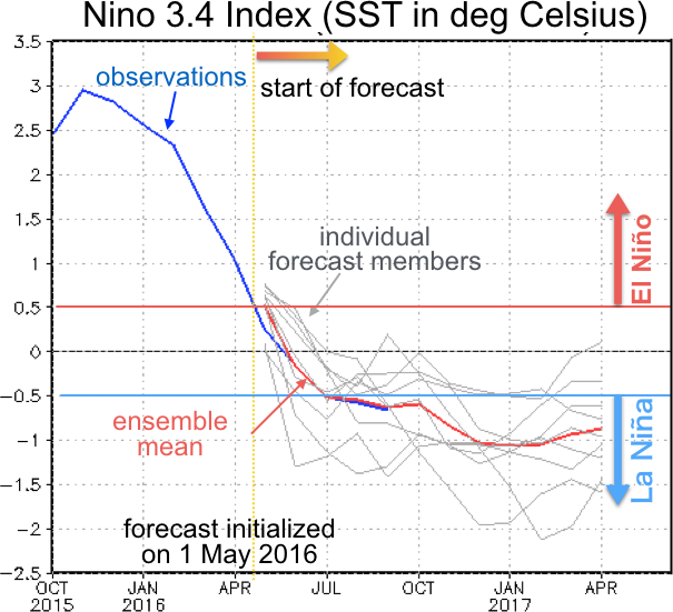
Let’s look at the El Niño forecast first. Figure 1 below shows how the Niño 3.4 index has evolved from October 2015 to present. The Niño 3.4 index is calculated by averaging sea-surface temperature (SST) anomalies over the eastern and central tropical Pacific, and it is one of the most important indicators for the state of the El Niño-Southern Oscillation (ENSO). The blue line shows the Niño 3.4 index as calculated from observations, which we take as our reference. From the end of 2015, El Niño started weakening and eventually terminated in May of 2016. Temperatures in the region continued to drop and weak La Niña-like conditions (the opposite phase of El Niño) settled in sometime in August or September. The red line shows the SINTEX-F forecast initialized from 1 May 2016. The match between the prediction and the observations is striking. This once more showcases the high skill of SINTEX-F in the tropical Pacific (previously documented, e.g., by Jin et al. 2008 in the journal Climate Dynamics).
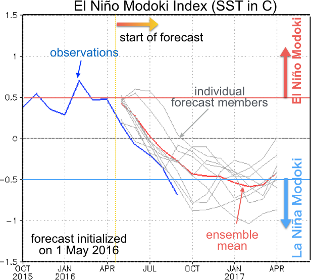
It was for a good reason that in the above I used the rather vague expression “La Niña-like conditions”. Only looking at the Niño 3.4 index hides the fact that this event is more typical of La Niña Modoki, where cool SST anomalies in the central equatorial Pacific are flanked by warm anomalies to the east and west. The Modoki character of this event is better documented by the El Niño Modoki Index (EMI; Fig. 2). The model prediction tracks the observed evolution from May rather well but tends to underestimate the amplitude, particularly in September (meaning that the predicted La Niña Modoki is too weak). A current APL research project funded by the Japanese Ministry of the Environment is working toward improving the prediction skill for phenomena like El Niño Modoki (grant number 2-1405: “Prediction of newly found climate phenomena and its societal application”, PI: Toshio Yamagata). I will probably write a post about the results of this project in the near future.
Because this summer was marked by the transition from El Niño to La Niña (or La Niña Modoki) SST anomalies in the tropical Pacific were rather small. In the tropical Indian Ocean, on the other hand, summer saw the development of a pronounced negative Indian Ocean Dipole (IOD) event that is still ongoing. This event probably played a major role in shaping the climate variations of this summer.
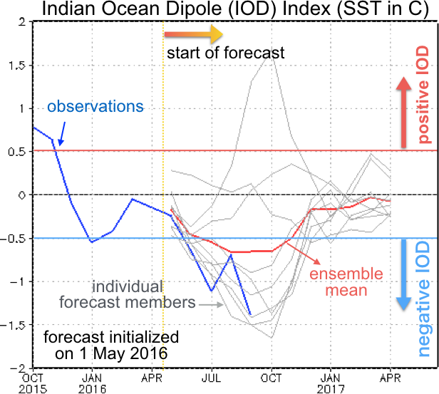
As shown by the Dipole Mode Index (DMI; Fig. 3), the negative IOD event rapidly developed in June and July, and kept going strongly in August and September. The SINTEX-F prediction did a reasonable job at predicting the development of the event, but severely underestimated its amplitude in July and September. Predicting the IOD is much harder than predicting El Niño. Exactly why that is the case is an area of current research, in which our lab (APL) is actively involved.
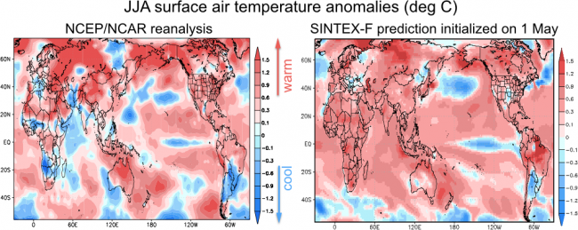
Next we take a look at the surface air temperature predictions. Figure 4 compares the surface air temperature anomalies in the NCEP/NCAR reanalysis (a product that combines observations and model simulation to obtain a best estimate of climate conditions) and the SINTEX-F predictions, both averaged from June through August. The model (right panel; initialized on 1 May) predicted warmer than average temperatures in most regions and, by and large, this is what actually occurred (according to the reanalysis data). For example, the predicted warm anomalies over northern Africa, Russia, China, northern America, Brazil and Australia are all validated by the reanalysis data. Unfortunately, the model was also wrong in a number of places, including southwestern Africa, parts of Europe, parts of India, and Japan’s Honshu (main) island.
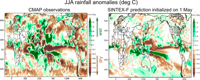
Finally, let’s look at rainfall. Figure 5 shows the CMAP observations (left panel) and the SINTEX-F prediction (initialized on 1 May), both averaged from June through August. There is good agreement between the observations and the SINTEX-F prediction over the tropical Pacific and Indian Ocean. The signature of the La Niña Modoki and negative IOD are well reproduced by the model. Over land, the heavy rain in Indonesia was well predicted (this was actually covered in the “Daily Jakarta Shimbun” newspaper). However, the rain shortage over North Brazil, the heavy rain over eastern Australia, and the precipitation distribution over the midlatitudes (including Japan) were not successfully predicted.
So what can we learn from shortcomings in the forecast? Successful prediction is rooted in the physical understanding of the underlying processes and their representation in numerical algorithms. Thus, if predictions fail it might indicate that there are still gaps in our knowledge of the physical mechanisms (though there can be other reasons as well). When you think about it this way, it can actually be exciting to examine why some predictions failed. Here at APL, we are actively working at better understanding the mechanisms of climate variations and improving our predictions accordingly. That includes examining the reasons for failed predictions, improving forecast techniques (e.g. modifying the model physics or initialization procedure). We are also looking at prediction from a more theoretical angle, e.g. by exploring the theoretical limits of prediction skill (aka predictability). We will probably report on some of those activities in the near future.
At the same time, APL is also working toward the practical application of forecast information for the benefit of society, e.g. by predicting crop yield or the outbreak of infectious diseases like malaria. If you would like to learn more about this, please check the following study on climate factors controlling Australian winter wheat yield (Japanese summary; link to article in Nature Scientific Reports) or this one on developing an early warning system for malaria in South Africa (Japanese; English/Japanese).
Finally, you can find the latest SINTEX-F forecast here [link to be added].